DCP Examples - Linear Programming (LP)
versioninfo()
using Convex, COSMO, CairoMakie, Gurobi, MathOptInterface, MosekTools, Random, SCS
const MOI = MathOptInterface
Linear programming (LP)
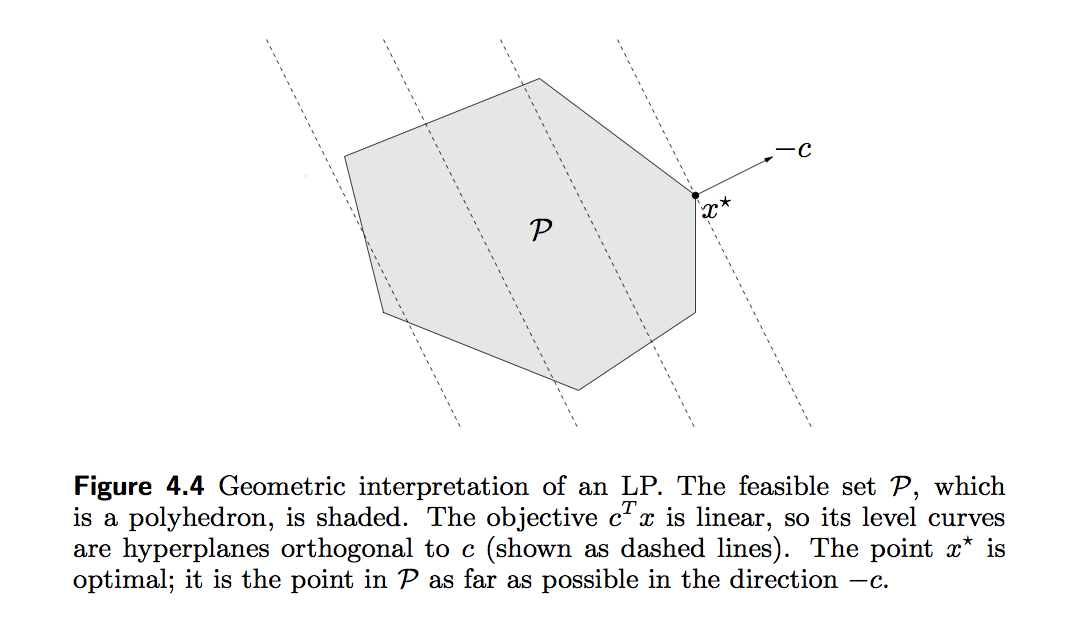
- A general linear program takes the form \begin{eqnarray*} &\text{minimize}& \mathbf{c}^T \mathbf{x} \\ &\text{subject to}& \mathbf{A} \mathbf{x} = \mathbf{b} \\ & & \mathbf{G} \mathbf{x} \preceq \mathbf{h}. \end{eqnarray*} Linear program is a convex optimization problem, why?
The standard form of an LP is \begin{eqnarray*} &\text{minimize}& \mathbf{c}^T \mathbf{x} \\ &\text{subject to}& \mathbf{A} \mathbf{x} = \mathbf{b} \\ & & \mathbf{x} \succeq \mathbf{0}. \end{eqnarray*} To transform a general linear program into the standard form, we introduce the slack variables $\mathbf{s} \succeq \mathbf{0}$ such that $\mathbf{G} \mathbf{x} + \mathbf{s} = \mathbf{h}$. Then we write $\mathbf{x} = \mathbf{x}^+ - \mathbf{x}^-$, where $\mathbf{x}^+ \succeq \mathbf{0}$ and $\mathbf{x}^- \succeq \mathbf{0}$. This yields the problem \begin{eqnarray*} &\text{minimize}& \mathbf{c}^T (\mathbf{x}^+ - \mathbf{x}^-) \\ &\text{subject to}& \mathbf{A} (\mathbf{x}^+ - \mathbf{x}^-) = \mathbf{b} \\ & & \mathbf{G} (\mathbf{x}^+ - \mathbf{x}^-) + \mathbf{s} = \mathbf{h} \\ & & \mathbf{x}^+ \succeq \mathbf{0}, \mathbf{x}^- \succeq \mathbf{0}, \mathbf{s} \succeq \mathbf{0} \end{eqnarray*} in $\mathbf{x}^+$, $\mathbf{x}^-$, and $\mathbf{s}$.
Slack variables are often used to transform a complicated inequality constraint to simple non-negativity constraints.
The inequality form of an LP is \begin{eqnarray*} &\text{minimize}& \mathbf{c}^T \mathbf{x} \\ &\text{subject to}& \mathbf{G} \mathbf{x} \preceq \mathbf{h}. \end{eqnarray*}
Some softwares, e.g.,
solveLPin R, require an LP be written in either standard or inequality form. However a good software should do this for you!A piecewise-linear minimization problem \begin{eqnarray*} &\text{minimize}& \max_{i=1,\ldots,m} (\mathbf{a}_i^T \mathbf{x} + b_i) \end{eqnarray*} can be transformed to an LP \begin{eqnarray*} &\text{minimize}& t \\ &\text{subject to}& \mathbf{a}_i^T \mathbf{x} + b_i \le t, \quad i = 1,\ldots,m, \end{eqnarray*} in $\mathbf{x}$ and $t$. Apparently $$ \text{minimize} \max_{i=1,\ldots,m} |\mathbf{a}_i^T \mathbf{x} + b_i| $$ and $$ \text{minimize} \max_{i=1,\ldots,m} (\mathbf{a}_i^T \mathbf{x} + b_i)_+ $$ are also LP.
Any convex optimization problem \begin{eqnarray*} &\text{minimize}& f_0(\mathbf{x}) \\ &\text{subject to}& f_i(\mathbf{x}) \le 0, \quad i=1,\ldots,m \\ && \mathbf{a}_i^T \mathbf{x} = b_i, \quad i=1,\ldots,p, \end{eqnarray*} where $f_0,\ldots,f_m$ are convex functions, can be transformed to the epigraph form \begin{eqnarray*} &\text{minimize}& t \\ &\text{subject to}& f_0(\mathbf{x}) - t \le 0 \\ & & f_i(\mathbf{x}) \le 0, \quad i=1,\ldots,m \\ & & \mathbf{a}_i^T \mathbf{x} = b_i, \quad i=1,\ldots,p \end{eqnarray*} in variables $\mathbf{x}$ and $t$. That is why people often say linear program is universal.
The linear fractional programming \begin{eqnarray*} &\text{minimize}& \frac{\mathbf{c}^T \mathbf{x} + d}{\mathbf{e}^T \mathbf{x} + f} \\ &\text{subject to}& \mathbf{A} \mathbf{x} = \mathbf{b} \\ & & \mathbf{G} \mathbf{x} \preceq \mathbf{h} \\ & & \mathbf{e}^T \mathbf{x} + f > 0 \end{eqnarray*} can be transformed to an LP \begin{eqnarray*} &\text{minimize}& \mathbf{c}^T \mathbf{y} + d z \\ &\text{subject to}& \mathbf{G} \mathbf{y} - z \mathbf{h} \preceq \mathbf{0} \\ & & \mathbf{A} \mathbf{y} - z \mathbf{b} = \mathbf{0} \\ & & \mathbf{e}^T \mathbf{y} + f z = 1 \\ & & z \ge 0 \end{eqnarray*} in $\mathbf{y}$ and $z$, via transformation of variables \begin{eqnarray*} \mathbf{y} = \frac{\mathbf{x}}{\mathbf{e}^T \mathbf{x} + f}, \quad z = \frac{1}{\mathbf{e}^T \mathbf{x} + f}. \end{eqnarray*} See Section 4.3.2 of Boyd and Vandenberghe (2004) for proof.
LP example: compressed sensing
- Compressed sensing Candes and Tao (2006) and Donoho (2006) tries to address a fundamental question: how to compress and transmit a complex signal (e.g., musical clips, mega-pixel images), which can be decoded to recover the original signal?

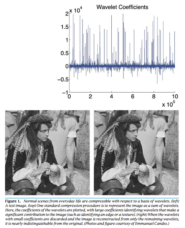
- Suppose a signal $\mathbf{x} \in \mathbb{R}^n$ is sparse with $s$ non-zeros. We under-sample the signal by multiplying a (flat) measurement matrix $\mathbf{y} = \mathbf{A} \mathbf{x}$, where $\mathbf{A} \in \mathbb{R}^{m\times n}$ has iid normal entries. Candes, Romberg and Tao (2006) show that the solution to \begin{eqnarray*} &\text{minimize}& \|\mathbf{x}\|_1 \\ &\text{subject to}& \mathbf{A} \mathbf{x} = \mathbf{y} \end{eqnarray*} exactly recovers the true signal under certain conditions on $\mathbf{A}$ when $n \gg s$ and $m \approx s \ln(n/s)$. Why sparsity is a reasonable assumption? Virtually all real-world images have low information content.
The $\ell_1$ minimization problem apparently is an LP, by writing $\mathbf{x} = \mathbf{x}^+ - \mathbf{x}^-$, \begin{eqnarray*} &\text{minimize}& \mathbf{1}^T (\mathbf{x}^+ + \mathbf{x}^-) \\ &\text{subject to}& \mathbf{A} (\mathbf{x}^+ - \mathbf{x}^-) = \mathbf{y} \\ & & \mathbf{x}^+ \succeq \mathbf{0}, \mathbf{x}^- \succeq \mathbf{0}. \end{eqnarray*}
Let's try a numerical example.
Generate a sparse signal and sub-sampling
# random seed
Random.seed!(123)
# Size of signal
n = 1024
# Sparsity (# nonzeros) in the signal
s = 20
# Number of samples (undersample by a factor of 8)
m = 128

# Generate and display the signal
x0 = zeros(n)
x0[rand(1:n, s)] = randn(s)
# Generate the random sampling matrix
A = randn(m, n) / m
# Subsample by multiplexing
y = A * x0

# plot the true signal
f = Figure()
Axis(
    f[1, 1],
    title = "True Signal x0",
    xlabel = "x",
    ylabel = "y"
)
lines!(1:n, x0)
f

Solve LP by DCP (disciplined convex programming) interface Convex.jl
Check Convex.jl documentation for a list of supported operations.
# # Use Mosek solver
# solver = Mosek.Optimizer()
# MOI.set(solver, MOI.RawOptimizerAttribute("LOG"), 1)

# # Use Gurobi solver
# solver = Gurobi.Optimizer()
# MOI.set(solver, MOI.RawOptimizerAttribute("OutputFlag"), 1)

# Use COSMO solver
solver = COSMO.Optimizer()
# MOI.set(solver, MOI.RawOptimizerAttribute("max_iter"), 5000)

# # Use SCS solver
# solver = SCS.Optimizer()
# MOI.set(solver, MOI.RawOptimizerAttribute("verbose"), 1)

# Set up optimizaiton problem
x = Variable(n)
problem = minimize(norm(x, 1))
problem.constraints += A * x == y

# Solve the problem
@time solve!(problem, solver)
# Display the solution
f = Figure()
Axis(
    f[1, 1],
    title = "Reconstructed signal overlayed with x0",
    xlabel = "x",
    ylabel = "y"
)
scatter!(1:n, x0, label = "truth")
lines!(1:n, vec(x.value), label = "recovery")
axislegend(position = :lt)
f

LP example: quantile regression
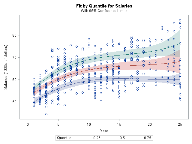
- In linear regression, we model the mean of response variable as a function of covariates. In many situations, the error variance is not constant, the distribution of $y$ may be asymmetric, or we simply care about the quantile(s) of response variable. Quantile regression offers a better modeling tool in these applications.
- In $\tau$-quantile regression, we minimize the loss function \begin{eqnarray*} f(\beta) = \sum_{i=1}^n \rho_\tau (y_i - \mathbf{x}_i^T \beta), \end{eqnarray*} where $\rho_\tau(z) = z (\tau - 1_{\{z < 0\}})$. Writing $\mathbf{y} - \mathbf{X} \beta = \mathbf{r}^+ - \mathbf{r}^-$, this is equivalent to the LP \begin{eqnarray*} &\text{minimize}& \tau \mathbf{1}^T \mathbf{r}^+ + (1-\tau) \mathbf{1}^T \mathbf{r}^- \\ &\text{subject to}& \mathbf{r}^+ - \mathbf{r}^- = \mathbf{y} - \mathbf{X} \beta \\ & & \mathbf{r}^+ \succeq \mathbf{0}, \mathbf{r}^- \succeq \mathbf{0} \end{eqnarray*} in $\mathbf{r}^+$, $\mathbf{r}^-$, and $\beta$.
LP Example: $\ell_1$ regression
A popular method in robust statistics is the median absolute deviation (MAD) regression that minimizes the $\ell_1$ norm of the residual vector $\|\mathbf{y} - \mathbf{X} \beta\|_1$. This apparently is equivalent to the LP \begin{eqnarray*} &\text{minimize}& \mathbf{1}^T (\mathbf{r}^+ + \mathbf{r}^-) \\ &\text{subject to}& \mathbf{r}^+ - \mathbf{r}^- = \mathbf{y} - \mathbf{X} \beta \\ & & \mathbf{r}^+ \succeq \mathbf{0}, \mathbf{r}^- \succeq \mathbf{0} \end{eqnarray*} in $\mathbf{r}^+$, $\mathbf{r}^-$, and $\beta$.
$\ell_1$ regression = MAD = 1/2-quantile regression.
LP Example: $\ell_\infty$ regression (Chebychev approximation)
- Minimizing the worst possible residual $\|\mathbf{y} - \mathbf{X} \beta\|_\infty$ is equivalent to the LP \begin{eqnarray*} &\text{minimize}& t \\ &\text{subject to}& -t \le y_i - \mathbf{x}_i^T \beta \le t, \quad i = 1,\dots,n \end{eqnarray*} in variables $\beta$ and $t$.
LP Example: Dantzig selector
- Candes and Tao (2007) propose a variable selection method called the Dantzig selector that solves \begin{eqnarray*} &\text{minimize}& \|\mathbf{X}^T (\mathbf{y} - \mathbf{X} \beta)\|_\infty \\ &\text{subject to}& \sum_{j=2}^p |\beta_j| \le t, \end{eqnarray*} which can be transformed to an LP. Indeed they name the method after George Dantzig, who invented the simplex method for efficiently solving LP in 50s.
LP Example: 1-norm SVM
- In two-class classification problems, we are given training data $(\mathbf{x}_i, y_i)$, $i=1,\ldots,n$, where $\mathbf{x}_i \in \mathbb{R}^p$ are feature vectors and $y_i \in \{-1, 1\}$ are class labels. Zhu, Rosset, Tibshirani, and Hastie (2004) propose the 1-norm support vector machine (svm) that achieves the dual purpose of classification and feature selection. Denote the solution of the optimization problem \begin{eqnarray*} &\text{minimize}& \sum_{i=1}^n \left[ 1 - y_i \left( \beta_0 + \sum_{j=1}^p x_{ij} \beta_j \right) \right]_+ \\ &\text{subject to}& \|\beta\|_1 = \sum_{j=1}^p |\beta_j| \le t \end{eqnarray*} by $\hat \beta_0(t)$ and $\hat \beta(t)$. 1-norm svm classifies a future feature vector $\mathbf{x}$ by the sign of fitted model \begin{eqnarray*} \hat f(\mathbf{x}) = \hat \beta_0 + \mathbf{x}^T \hat \beta. \end{eqnarray*}
Many more applications of LP: Airport scheduling (Copenhagen airport uses Gurobi), airline flight scheduling, NFL scheduling, match.com, $\LaTeX$, ...
Apparently any loss/penalty or loss/constraint combinations of form $$ \{\ell_1, \ell_\infty, \text{quantile}\} \times \{\ell_1, \ell_\infty, \text{quantile}\}, $$ possibly with affine (equality and/or inequality) constraints, can be formulated as an LP.