Optimization in Julia
This lecture gives an overview of some optimization tools in Julia.
versioninfo()
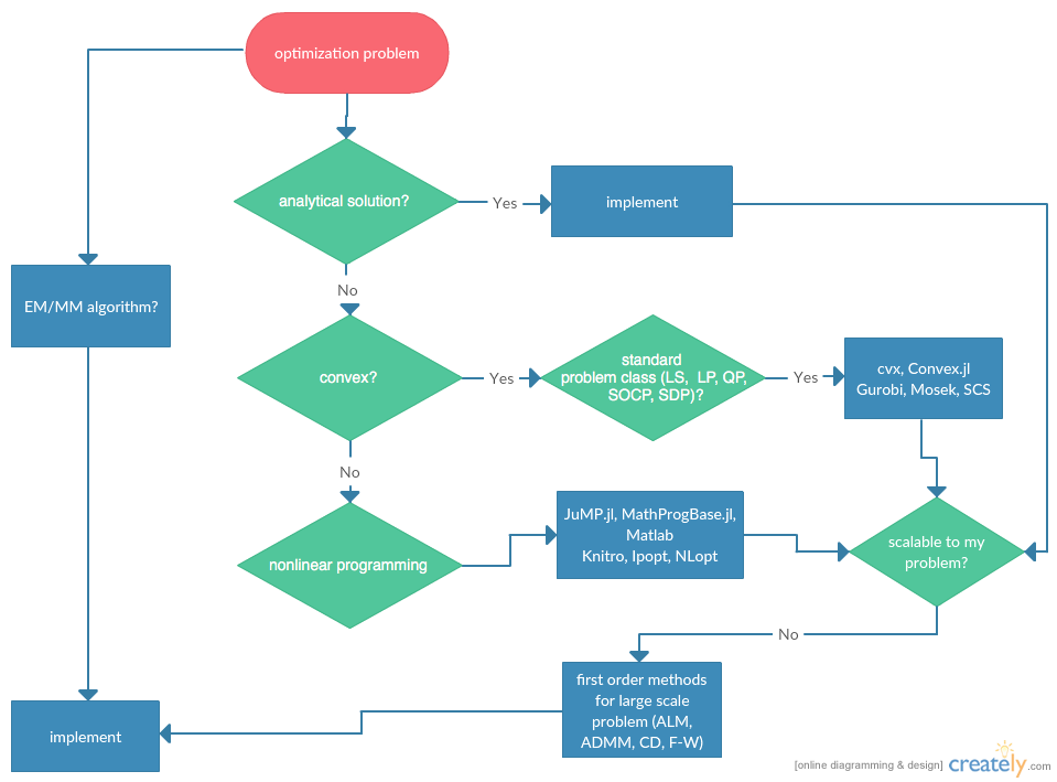
Flowchart
Statisticians do optimizations in daily life: maximum likelihood estimation, machine learning, ...
Category of optimization problems:
Problems with analytical solutions: least squares, principle component analysis, canonical correlation analysis, ...
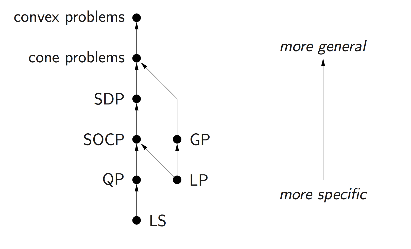
Problems subject to Disciplined Convex Programming (DCP): linear programming (LP), quadratic programming (QP), second-order cone programming (SOCP), semidefinite programming (SDP), and geometric programming (GP).
Nonlinear programming (NLP): Newton type algorithms, Fisher scoring algorithm, EM algorithm, MM algorithms.
Large scale optimization: ADMM, SGD, ...
Modeling tools and solvers
Getting familiar with good optimization softwares broadens the scope and scale of problems we are able to solve in statistics. Following table lists some of the best optimization softwares.
| LP | MILP | SOCP | MISOCP | SDP | GP | NLP | MINLP | R | Matlab | Julia | Python | Cost | ||||
|---|---|---|---|---|---|---|---|---|---|---|---|---|---|---|---|---|
| modeling tools | ||||||||||||||||
| cvx | x | x | x | x | x | x | x | x | x | A | ||||||
| Convex.jl | x | x | x | x | x | x | O | |||||||||
| JuMP.jl | x | x | x | x | x | x | x | O | ||||||||
| MathProgBase.jl | x | x | x | x | x | x | x | O | ||||||||
| MathOptInterface.jl | x | x | x | x | x | x | x | O | ||||||||
| convex solvers | ||||||||||||||||
| Mosek | x | x | x | x | x | x | x | x | x | x | x | A | ||||
| Gurobi | x | x | x | x | x | x | x | x | A | |||||||
| CPLEX | x | x | x | x | x | x | x | x | A | |||||||
| SCS | x | x | x | x | x | x | O | |||||||||
| COSMO.jl | x | x | x | x | O | |||||||||||
| NLP solvers | ||||||||||||||||
| NLopt | x | x | x | x | x | x | O | |||||||||
| Ipopt | x | x | x | x | x | x | O | |||||||||
| KNITRO | x | x | x | x | x | x | x | x | $ |
- O: open source
- A: free academic license
- $: commercial
Difference between modeling tool and solvers
Modeling tools such as cvx (for Matlab) and Convex.jl (Julia analog of cvx) implement the disciplined convex programming (DCP) paradigm proposed by Grant and Boyd (2008) http://stanford.edu/~boyd/papers/disc_cvx_prog.html. DCP prescribes a set of simple rules from which users can construct convex optimization problems easily.
Solvers (Mosek, Gurobi, Cplex, SCS, COSMO, ...) are concrete software implementation of optimization algorithms. My favorite ones are: Mosek/Gurobi/SCS for DCP and Ipopt/NLopt for nonlinear programming. Mosek and Gurobi are commercial software but free for academic use. SCS/Ipopt/NLopt are open source.
Modeling tools usually have the capability to use a variety of solvers. But modeling tools are solver agnostic so users do not have to worry about specific solver interface.
For this course, install following tools:
- Gurobi: 1. Download Gurobi at link. 2. Request free academic license at link. 3. Run
grbgetkey XXXXXXXXXcommand on terminal as suggested. It'll retrieve a license file and put it under the home folder. 4. Set up the environmental variables. On my machine, I put following two lines in the~/.julia/config/startup.jlfile:ENV["GUROBI_HOME"] = "/Library/gurobi902/mac64"andENV["GRB_LICENSE_FILE"] = "/Users/huazhou/Documents/Gurobi/gurobi.lic". - Mosek: 1. Request free academic license at link. The license file will be sent to your edu email within minutes. Check Spam folder if necessary. 2. Put the license file at the default location
~/mosek/. - Convex.jl, SCS.jl, Gurobi.jl, Mosek.jl, MathProgBase.jl, NLopt.jl, Ipopt.jl.
- Gurobi: 1. Download Gurobi at link. 2. Request free academic license at link. 3. Run
DCP Using Convex.jl
Standard convex problem classes like LP (linear programming), QP (quadratic programming), SOCP (second-order cone programming), SDP (semidefinite programming), and GP (geometric programming), are becoming a technology.
Example: microbiome regression analysis
We illustrate optimization tools in Julia using microbiome analysis as an example.
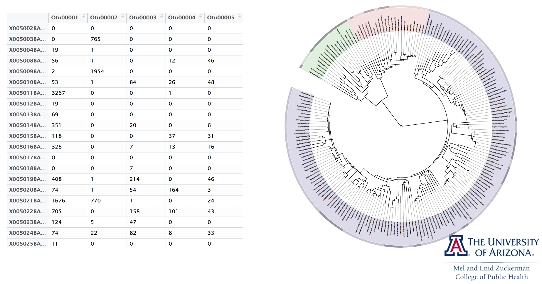
16S microbiome sequencing techonology generates sequence counts of various organisms (OTUs, operational taxonomic units) in samples.
For statistical analysis, counts are normalized into proportions for each sample, resulting in a covariate matrix $\mathbf{X}$ with all rows summing to 1. For identifiability, we need to add a sum-to-zero constraint to the regression cofficients. In other words, we need to solve a constrained least squares problem
$$
\text{minimize} \frac{1}{2} \|\mathbf{y} - \mathbf{X} \beta\|_2^2
$$
subject to the constraint $\sum_{j=1}^p \beta_j = 0$. For simplicity we ignore intercept and non-OTU covariates in this presentation.
Let's first generate an artifical data set.
using Random, LinearAlgebra, SparseArrays

Random.seed!(257) # seed

n, p = 100, 50
X = rand(n, p)
# scale each row of X sum to 1
lmul!(Diagonal(1 ./ vec(sum(X, dims=2))), X)
# true β is a sparse vector with about 10% non-zero entries
β = sprandn(p, 0.1)
y = X * β + randn(n);
Sum-to-zero regression
The sum-to-zero contrained least squares is a standard quadratic programming (QP) problem so should be solved easily by any QP solver.
Modeling using Convex.jl
We use the Convex.jl package to model this QP problem. For a complete list of operations supported by Convex.jl, see http://www.juliaopt.org/Convex.jl/stable/operations/.
using Convex

β̂cls = Variable(size(X, 2))
problem = minimize(0.5sumsquares(y - X * β̂cls)) # objective
problem.constraints += sum(β̂cls) == 0; # constraint
problem
Mosek
We first use the Mosek solver to solve this QP.
using MosekTools, MathOptInterface
const MOI = MathOptInterface

#solver = Model(optimizer_with_attributes(Mosek.Optimizer, "LOG" => 1))
solver = Mosek.Optimizer()
MOI.set(solver, MOI.RawOptimizerAttribute("LOG"), 1)

@time solve!(problem, solver)
# Check the status, optimal value, and minimizer of the problem
problem.status, problem.optval, β̂cls.value
# check constraint satisfication
sum(β̂cls.value)
Gurobi
Switch to Gurobi solver:
using Gurobi
solver = Gurobi.Optimizer()
MOI.set(solver, MOI.RawOptimizerAttribute("OutputFlag"), 1)

@time solve!(problem, solver)
# Check the status, optimal value, and minimizer of the problem
problem.status, problem.optval, β̂cls.value
# check constraint satisfication
sum(β̂cls.value)
COSMO
Switch to COSMO solver (pure Julia implementation):
# Use COSMO solver
using COSMO

solver = COSMO.Optimizer()
MOI.set(solver, MOI.RawOptimizerAttribute("max_iter"), 5000)

@time solve!(problem, solver)
# Check the status, optimal value, and minimizer of the problem
problem.status, problem.optval, β̂cls.value
We see COSMO have a looser criterion for constraint satisfication, resulting a lower objective value.
sum(β̂cls.value)
SCS
Switch to the open source SCS solver:
# Use SCS solver
using SCS

solver = SCS.Optimizer()
MOI.set(solver, MOI.RawOptimizerAttribute("verbose"), 1)

@time solve!(problem, solver)
# Check the status, optimal value, and minimizer of the problem
problem.status, problem.optval, β̂cls.value
# check constraint satisfication
sum(β̂cls.value)
Sum-to-zero lasso
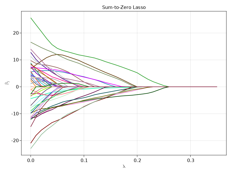
Suppose we want to know which organisms (OTU) are associated with the response. We can answer this question using a sum-to-zero contrained lasso $$ \text{minimize} \frac 12 \|\mathbf{y} - \mathbf{X} \beta\|_2^2 + \lambda \|\beta\|_1 $$ subject to the constraint $\sum_{j=1}^p \beta_j = 0$. Varying $\lambda$ from small to large values will generate a solution path.
using Convex

# # Use Mosek solver
# using Mosek
# solver = Mosek.Optimizer()
# MOI.set(solver, MOI.RawOptimizerAttribute("LOG"), 0)

# # Use Gurobi solver
# using Gurobi
# solver = () -> Gurobi.Optimizer(OutputFlag=0)

# Use Cplex solver
# using CPLEX
# solver = CplexSolver(CPXPARAM_ScreenOutput=0)

# # Use SCS solver
# using SCS
# solver = () -> SCS.Optimizer(verbose=0)

# solve at a grid of λ
λgrid = 0:0.01:0.35

# holder for solution path
β̂path = zeros(length(λgrid), size(X, 2)) # each row is β̂ at a λ
# optimization variable
β̂classo = Variable(size(X, 2))
# obtain solution path using warm start
@time for i in 1:length(λgrid)
    λ = λgrid[i]
    # define optimization problem
    # objective
    problem = minimize(0.5sumsquares(y - X * β̂classo) + λ * sum(abs, β̂classo))
    # constraint
    problem.constraints += sum(β̂classo) == 0 # constraint
    solver = Mosek.Optimizer()
    MOI.set(solver, MOI.RawOptimizerAttribute("LOG"), 0)
    solve!(problem, solver)
    β̂path[i, :] = β̂classo.value
end
using CairoMakie

f = Figure()
Axis(
    f[1, 1],
    title = "Sum-to-Zero Lasso",
    xlabel = L"\lambda",
    ylabel = L"\beta_j"
)
series!(λgrid, β̂path', color = :glasbey_category10_n256)
f
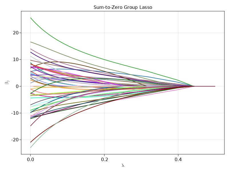
Sum-to-zero group lasso
Suppose we want to do variable selection not at the OTU level, but at the Phylum level. OTUs are clustered into various Phyla. We can answer this question using a sum-to-zero contrained group lasso $$ \text{minimize} \frac 12 \|\mathbf{y} - \mathbf{X} \beta\|_2^2 + \lambda \sum_j \|\mathbf{\beta}_j\|_2 $$ subject to the constraint $\sum_{j=1}^p \beta_j = 0$, where $\mathbf{\beta}_j$ are regression coefficients corresponding to the $j$-th phylum. This is a second-order cone programming (SOCP) problem readily modeled by Convex.jl.
Let's assume each 10 contiguous OTUs belong to one Phylum.
# Use Mosek solver
using MosekTools

# # Use Gurobi solver
# using Gurobi

# # Use Cplex solver
# using CPLEX
# solver = CplexSolver(CPXPARAM_ScreenOutput=0)

# # Use SCS solver
# using SCS
# solver = SCSSolver(verbose=0)

# solve at a grid of λ
λgrid = 0.0:0.005:0.5
β̂pathgrp = zeros(length(λgrid), size(X, 2)) # each row is β̂ at a λ
β̂classo = Variable(size(X, 2))
@time for i in 1:length(λgrid)
    λ = λgrid[i]
    # loss
    obj = 0.5sumsquares(y - X * β̂classo)
    # group lasso penalty term
    for j in 1:(size(X, 2)/10)
        βj = β̂classo[(10(j-1)+1):10j]
        obj = obj + λ * norm(βj)
    end
    problem = minimize(obj)
    # constraint
    problem.constraints += sum(β̂classo) == 0 # constraint
    solver = Mosek.Optimizer()
    MOI.set(solver, MOI.RawOptimizerAttribute("LOG"), 0)
    solve!(problem, solver)
    β̂pathgrp[i, :] = β̂classo.value
end
We see it took Mosek <2 second to solve this seemingly hard optimization problem at 101 different $\lambda$ values.
using CairoMakie

f = Figure()
Axis(
    f[1, 1],
    title = "Sum-to-Zero Group Lasso",
    xlabel = L"\lambda",
    ylabel = L"\beta_j"
)
series!(λgrid, β̂pathgrp', color = :glasbey_category10_n256)
f
Example: matrix completion
Load the $128 \times 128$ Lena picture with missing pixels.
using FileIO

lena = load("lena128missing.png")

# convert to real matrices
Y = Float64.(lena)
We fill out the missin pixels uisng a matrix completion technique developed by Candes and Tao $$ \text{minimize } \|\mathbf{X}\|_* $$ $$ \text{subject to } x_{ij} = y_{ij} \text{ for all observed entries } (i, j). $$ Here $\|\mathbf{M}\|_* = \sum_i \sigma_i(\mathbf{M})$ is the nuclear norm. In words we seek the matrix with minimal nuclear norm that agrees with the observed entries. This is a semidefinite programming (SDP) problem readily modeled by Convex.jl.
This example takes long because of high dimensionality.
# Use COSMO solver
using COSMO

# Linear indices of obs. entries
obsidx = findall(Y[:] .≠ 0.0)
# Create optimization variables
X = Variable(size(Y))
# Set up optmization problem
problem = minimize(nuclearnorm(X))
problem.constraints += X[obsidx] == Y[obsidx]
# Solve the problem by calling solve
# @time solve!(problem, () -> Mosek.Optimizer(LOG=1)) # Mosek takes about 20min
@time solve!(problem, COSMO.Optimizer()) # fast
using Images

#Gray.(X.value)
colorview(Gray, X.value)

Nonlinear programming (NLP)
We use MLE of Gamma distribution to illustrate some rudiments of nonlinear programming (NLP) in Julia.
Let $x_1,\ldots,x_m$ be a random sample from the gamma density $$ f(x) = \Gamma(\alpha)^{-1} \beta^{\alpha} x^{\alpha-1} e^{-\beta x} $$ on $(0,\infty)$. The loglikelihood function is $$ L(\alpha, \beta) = m [- \ln \Gamma(\alpha) + \alpha \ln \beta + (\alpha - 1)\overline{\ln x} - \beta \bar x], $$ where $\overline{x} = \frac{1}{m} \sum_{i=1}^m x_i$ and $\overline{\ln x} = \frac{1}{m} \sum_{i=1}^m \ln x_i$.
using Random, Statistics, SpecialFunctions
Random.seed!(123)

function gamma_logpdf(x::Vector, α::Real, β::Real)
    m = length(x)
    avg = mean(x)
    logavg = sum(log, x) / m
    m * (- log(gamma(α)) + α * log(β) + (α - 1) * logavg - β * avg)
end

x = rand(5)
gamma_logpdf(x, 1.0, 1.0)
Many optimization algorithms involve taking derivatives of the objective function. The ForwardDiff.jl package implements automatic differentiation. For example, to compute the derivative and Hessian of the log-likelihood with data x at α=1.0 and β=1.0.
using ForwardDiff

ForwardDiff.gradient(θ -> gamma_logpdf(x, θ...), [1.0; 1.0])
ForwardDiff.hessian(θ -> gamma_logpdf(x, θ...), [1.0; 1.0])
Generate data:
using Distributions, Random

Random.seed!(123)
(n, p) = (1000, 2)
(α, β) = 5.0 * rand(p)
x = rand(Gamma(α, β), n)
println("True parameter values:")
println("α = ", α, ", β = ", β)
We use JuMP.jl to define and solve our NLP problem.
using JuMP

# using NLopt
# m = Model(NLopt.Optimizer)
# set_optimizer_attribute(m, "algorithm", :LD_MMA)

using Ipopt
m = Model(Ipopt.Optimizer)
set_optimizer_attribute(m, "print_level", 3)

myf(a, b) = gamma_logpdf(x, a, b)
JuMP.register(m, :myf, 2, myf, autodiff=true)
@variable(m, α >= 1e-8)
@variable(m, β >= 1e-8)
@NLobjective(m, Max, myf(α, β))

print(m)
status = JuMP.optimize!(m)

println("MLE (JuMP):")
println("α = ", α, ", β = ", β)
println("Objective value: ", JuMP.objective_value(m))
println("α = ", JuMP.value(α), ", β = ", 1 / JuMP.value(β))
println("MLE (Distribution package):")
println(fit_mle(Gamma, x))