Conjugate Gradient and Krylov Subspace Methods

In [1]:
versioninfo()
Julia Version 1.7.1
Commit ac5cc99908 (2021-12-22 19:35 UTC)
Platform Info:
  OS: macOS (x86_64-apple-darwin19.5.0)
  CPU: Intel(R) Core(TM) i7-6920HQ CPU @ 2.90GHz
  WORD_SIZE: 64
  LIBM: libopenlibm
  LLVM: libLLVM-12.0.1 (ORCJIT, skylake)
Environment:
  JULIA_EDITOR = code
  JULIA_NUM_THREADS = 4

Introduction

  • Conjugate gradient is the top-notch iterative method for solving large, structured linear systems $\mathbf{A} \mathbf{x} = \mathbf{b}$, where $\mathbf{A}$ is pd.
    Earlier we talked about Jacobi, Gauss-Seidel, and successive over-relaxation (SOR) as the classical iterative solvers. They are rarely used in practice due to slow convergence.

    Kershaw's results for a fusion problem.

Method Number of Iterations
Gauss Seidel 208,000
Block SOR methods 765
Incomplete Cholesky conjugate gradient 25
  • History: Hestenes (UCLA professor!) and Stiefel proposed conjugate gradient method in 1950s.

Hestenes and Stiefel (1952), Methods of conjugate gradients for solving linear systems, Jounral of Research of the National Bureau of Standards.

  • Solve linear equation $\mathbf{A} \mathbf{x} = \mathbf{b}$, where $\mathbf{A} \in \mathbb{R}^{n \times n}$ is pd, is equivalent to $$ \begin{eqnarray*} \text{minimize} \,\, f(\mathbf{x}) = \frac 12 \mathbf{x}^T \mathbf{A} \mathbf{x} - \mathbf{b}^T \mathbf{x}. \end{eqnarray*} $$ Denote $\nabla f(\mathbf{x}) = \mathbf{A} \mathbf{x} - \mathbf{b} =: r(\mathbf{x})$.

Conjugate gradient (CG) method

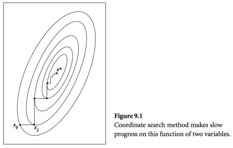
  • Consider a simple idea: coordinate descent, that is to update components $x_j$ alternatingly. Same as the Gauss-Seidel iteration. Usually it takes too many iterations.

  • A set of vectors $\{\mathbf{p}^{(0)},\ldots,\mathbf{p}^{(l)}\}$ is said to be conjugate with respect to $\mathbf{A}$ if $$ \begin{eqnarray*} \mathbf{p}_i^T \mathbf{A} \mathbf{p}_j = 0, \quad \text{for all } i \ne j. \end{eqnarray*} $$ For example, eigen-vectors of $\mathbf{A}$ are conjugate to each other. Why?

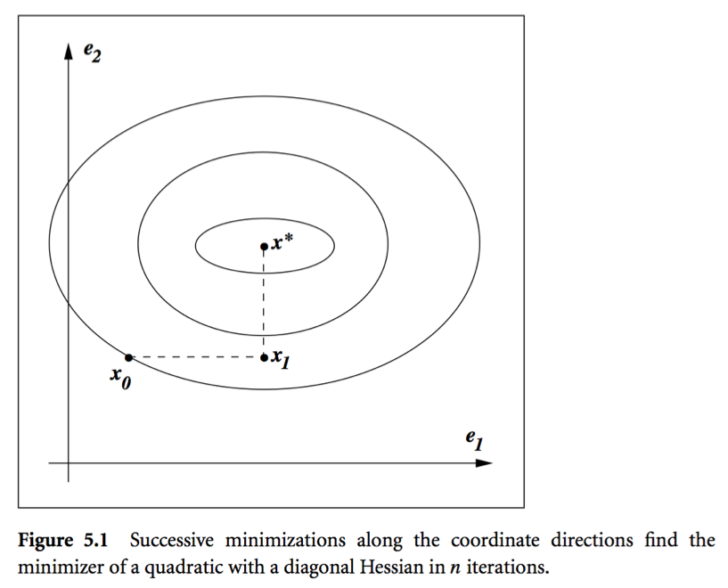
  • Conjugate direction method: Given a set of conjugate vectors $\{\mathbf{p}^{(0)},\ldots,\mathbf{p}^{(l)}\}$, at iteration $t$, we search along the conjugate direction $\mathbf{p}^{(t)}$ $$ \begin{eqnarray*} \mathbf{x}^{(t+1)} = \mathbf{x}^{(t)} + \alpha^{(t)} \mathbf{p}^{(t)}, \end{eqnarray*} $$ where $$ \begin{eqnarray*} \alpha^{(t)} = - \frac{\mathbf{r}^{(t)T} \mathbf{p}^{(t)}}{\mathbf{p}^{(t)T} \mathbf{A} \mathbf{p}^{(t)}} \end{eqnarray*} $$ is the optimal step length.

  • Theorem: In conjugate direction method, $\mathbf{x}^{(t)}$ converges to the solution in at most $n$ steps.

    Intuition: Look at graph.

  • Conjugate gradient method. Idea: generate $\mathbf{p}^{(t)}$ using only $\mathbf{p}^{(t-1)}$ $$ \begin{eqnarray*} \mathbf{p}^{(t)} = - \mathbf{r}^{(t)} + \beta^{(t)} \mathbf{p}^{(t-1)}, \end{eqnarray*} $$ where $\beta^{(t)}$ is determined by the conjugacy condition $\mathbf{p}^{(t-1)T} \mathbf{A} \mathbf{p}^{(t)} = 0$ $$ \begin{eqnarray*} \beta^{(t)} = \frac{\mathbf{r}^{(t)T} \mathbf{A} \mathbf{p}^{(t-1)}}{\mathbf{p}^{(t-1)T} \mathbf{A} \mathbf{p}^{(t-1)}}. \end{eqnarray*} $$

  • CG algorithm (preliminary version):

    1. Given $\mathbf{x}^{(0)}$
    2. Initialize: $\mathbf{r}^{(0)} \gets \mathbf{A} \mathbf{x}^{(0)} - \mathbf{b}$, $\mathbf{p}^{(0)} \gets - \mathbf{r}^{(0)}$, $t=0$
    3. While $\mathbf{r}^{(0)} \ne \mathbf{0}$

      1. $\alpha^{(t)} \gets - \frac{\mathbf{r}^{(t)T} \mathbf{p}^{(t)}}{\mathbf{p}^{(t)T} \mathbf{A} \mathbf{p}^{(t)}}$
      2. $\mathbf{x}^{(t+1)} \gets \mathbf{x}^{(t)} + \alpha^{(t)} \mathbf{p}^{(t)}$
      3. $\mathbf{r}^{(t+1)} \gets \mathbf{A} \mathbf{x}^{(t+1)} - \mathbf{b}$
      4. $\beta^{(t+1)} \gets \frac{\mathbf{r}^{(t+1)T} \mathbf{A} \mathbf{p}^{(t)}}{\mathbf{p}^{(t)T} \mathbf{A} \mathbf{p}^{(t)}}$
      5. $\mathbf{p}^{(t+1)} \gets - \mathbf{r}^{(t+1)} + \beta^{(t+1)} \mathbf{p}^{(t)}$
      6. $t \gets t+1$

      Remark: The initial conjugate direction $\mathbf{p}^{(0)} \gets - \mathbf{r}^{(0)}$ is crucial.

  • Theorem: With CG algorithm

    1. $\mathbf{r}^{(t)}$ are mutually orthogonal.
    2. $\{\mathbf{r}^{(0)},\ldots,\mathbf{r}^{(t)}\}$ is contained in the Krylov subspace of degree $t$ for $\mathbf{r}^{(0)}$, denoted by $$ \begin{eqnarray*} {\cal K}(\mathbf{r}^{(0)}; t) = \text{span} \{\mathbf{r}^{(0)},\mathbf{A} \mathbf{r}^{(0)}, \mathbf{A}^2 \mathbf{r}^{(0)}, \ldots, \mathbf{A}^{t} \mathbf{r}^{(0)}\}. \end{eqnarray*} $$
    3. $\{\mathbf{p}^{(0)},\ldots,\mathbf{p}^{(t)}\}$ is contained in ${\cal K}(\mathbf{r}^{(0)}; t)$.
    4. $\mathbf{p}^{(0)}, \ldots, \mathbf{p}^{(t)}$ are conjugate with respect to $\mathbf{A}$.
      The iterates $\mathbf{x}^{(t)}$ converge to the solution in at most $n$ steps.
  • CG algorithm (economical version): saves one matrix-vector multiplication.

    1. Given $\mathbf{x}^{(0)}$
    2. Initialize: $\mathbf{r}^{(0)} \gets \mathbf{A} \mathbf{x}^{(0)} - \mathbf{b}$, $\mathbf{p}^{(0)} \gets - \mathbf{r}^{(0)}$, $t=0$
    3. While $\mathbf{r}^{(0)} \ne \mathbf{0}$
      1. $\alpha^{(t)} \gets \frac{\mathbf{r}^{(t)T} \mathbf{r}^{(t)}}{\mathbf{p}^{(t)T} \mathbf{A} \mathbf{p}^{(t)}}$
      2. $\mathbf{x}^{(t+1)} \gets \mathbf{x}^{(t)} + \alpha^{(t)} \mathbf{p}^{(t)}$
      3. $\mathbf{r}^{(t+1)} \gets \mathbf{r}^{(t)} + \alpha^{(t)} \mathbf{A} \mathbf{p}^{(t)}$
      4. $\beta^{(t+1)} \gets \frac{\mathbf{r}^{(t+1)T} \mathbf{r}^{(t+1)}}{\mathbf{r}^{(t)T} \mathbf{r}^{(t)}}$
      5. $\mathbf{p}^{(t+1)} \gets - \mathbf{r}^{(t+1)} + \beta^{(t+1)} \mathbf{p}^{(t)}$
      6. $t \gets t+1$
  • Computation cost per iteration is one matrix vector multiplication: $\mathbf{A} \mathbf{p}^{(t)}$.
    Consider PageRank problem, $\mathbf{A}$ has dimension $n \approx 10^{10}$ but is highly structured (sparse + low rank). Each matrix vector multiplication takes $O(n)$.

  • Theorem: If $\mathbf{A}$ has $r$ distinct eigenvalues, $\mathbf{x}^{(t)}$ converges to solution $\mathbf{x}^*$ in at most $r$ steps.

Pre-conditioned conjugate gradient (PCG)

  • Summary of conjugate gradient method for solving $\mathbf{A} \mathbf{x} = \mathbf{b}$ or equivalently minimizing $\frac 12 \mathbf{x}^T \mathbf{A} \mathbf{x} - \mathbf{b}^T \mathbf{x}$:

    • Each iteration needs one matrix vector multiplication: $\mathbf{A} \mathbf{p}^{(t+1)}$. For structured $\mathbf{A}$, often $O(n)$ cost per iteration.
    • Guaranteed to converge in $n$ steps.
  • Two important bounds for conjugate gradient algorithm:

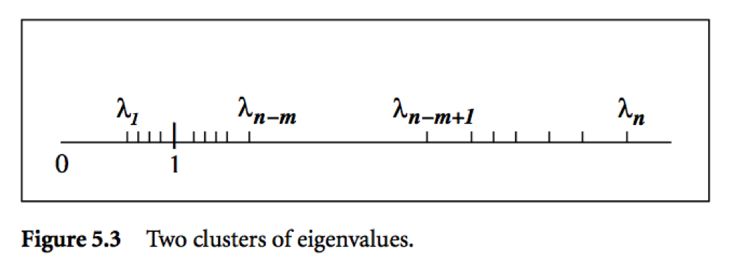
    Let $\lambda_1 \le \cdots \le \lambda_n$ be the ordered eigenvalues of a pd $\mathbf{A}$.
    $$ \begin{eqnarray*} \|\mathbf{x}^{(t+1)} - \mathbf{x}^*\|_{\mathbf{A}}^2 &\le& \left( \frac{\lambda_{n-t} - \lambda_1}{\lambda_{n-t} + \lambda_1} \right)^2 \|\mathbf{x}^{(0)} - \mathbf{x}^*\|_{\mathbf{A}}^2 \\ \|\mathbf{x}^{(t+1)} - \mathbf{x}^*\|_{\mathbf{A}}^2 &\le& 2 \left( \frac{\sqrt{\kappa(\mathbf{A})}-1}{\sqrt{\kappa(\mathbf{A})}+1} \right)^{t} \|\mathbf{x}^{(0)} - \mathbf{x}^*\|_{\mathbf{A}}^2, \end{eqnarray*} $$ where $\kappa(\mathbf{A}) = \lambda_n/\lambda_1$ is the condition number of $\mathbf{A}$.
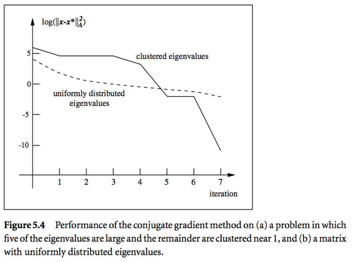
  • Messages:

    • Roughly speaking, if the eigenvalues of $\mathbf{A}$ occur in $r$ distinct clusters, the CG iterates will approximately solve the problem after $O(r)$ steps.
    • $\mathbf{A}$ with a small condition number ($\lambda_1 \approx \lambda_n$) converges fast.
  • Pre-conditioning: Change of variables $\widehat{\mathbf{x}} = \mathbf{C} \mathbf{x}$ via a nonsingular $\mathbf{C}$ and solve $$ (\mathbf{C}^{-T} \mathbf{A} \mathbf{C}^{-1}) \widehat{\mathbf{x}} = \mathbf{C}^{-T} \mathbf{b}. $$ Choose $\mathbf{C}$ such that

    • $\mathbf{C}^{-T} \mathbf{A} \mathbf{C}^{-1}$ has small condition number, or
    • $\mathbf{C}^{-T} \mathbf{A} \mathbf{C}^{-1}$ has clustered eigenvalues
    • Inexpensive solution of $\mathbf{C}^T \mathbf{C} \mathbf{y} = \mathbf{r}$
  • Preconditioned CG does not make use of $\mathbf{C}$ explicitly, but rather the matrix $\mathbf{M} = \mathbf{C}^T \mathbf{C}$.

  • Preconditioned CG (PCG) algorithm:

    1. Given $\mathbf{x}^{(0)}$, pre-conditioner $\mathbf{M}$
    2. $\mathbf{r}^{(0)} \gets \mathbf{A} \mathbf{x}^{(0)} - \mathbf{b}$
    3. solve $\mathbf{M} \mathbf{y}^{(0)} = \mathbf{r}^{(0)}$ for $\mathbf{y}^{(0)}$
    4. $\mathbf{p}^{(0)} \gets - \mathbf{r}^{(0)}$, $t=0$
    5. While $\mathbf{r}^{(0)} \ne \mathbf{0}$

      1. $\alpha^{(t)} \gets \frac{\mathbf{r}^{(t)T} \mathbf{y}^{(t)}}{\mathbf{p}^{(t)T} \mathbf{A} \mathbf{p}^{(t)}}$
      2. $\mathbf{x}^{(t+1)} \gets \mathbf{x}^{(t)} + \alpha^{(t)} \mathbf{p}^{(t)}$
      3. $\mathbf{r}^{(t+1)} \gets \mathbf{r}^{(t)} + \alpha^{(t)} \mathbf{A} \mathbf{p}^{(t)}$
      4. Solve $\mathbf{M} \mathbf{y}^{(t+1)} \gets \mathbf{r}^{(t+1)}$ for $\mathbf{y}^{(t+1)}$
      5. $\beta^{(t+1)} \gets \frac{\mathbf{r}^{(t+1)T} \mathbf{y}^{(t+1)}}{\mathbf{r}^{(t)T} \mathbf{r}^{(t)}}$
      6. $\mathbf{p}^{(t+1)} \gets - \mathbf{y}^{(t+1)} + \beta^{(t+1)} \mathbf{p}^{(t)}$
      7. $t \gets t+1$

      Remark: Only extra cost in the pre-conditioned CG algorithm is the need to solve the linear system $\mathbf{M} \mathbf{y} = \mathbf{r}$.

  • Pre-conditioning is more like an art than science. Some choices include

    • Incomplete Cholesky. $\mathbf{A} \approx \tilde{\mathbf{L}} \tilde{\mathbf{L}}^T$, where $\tilde{\mathbf{L}}$ is a sparse approximate Cholesky factor. Then $\tilde{\mathbf{L}}^{-1} \mathbf{A} \tilde{\mathbf{L}}^{-T} \approx \mathbf{I}$ (perfectly conditioned) and $\mathbf{M} \mathbf{y} = \tilde{\mathbf{L}} \tilde {\mathbf{L}}^T \mathbf{y} = \mathbf{r}$ is easy to solve.
    • Banded pre-conditioners.
    • Choose $\mathbf{M}$ as a coarsened version of $\mathbf{A}$.
    • Subject knowledge. Knowledge about the structure and origin of a problem is often the key to devising efficient pre-conditioner. For example, see recent work of Stein, Chen, Anitescu (2012) for pre-conditioning large covariance matrices. http://epubs.siam.org/doi/abs/10.1137/110834469

Example of PCG

Preconditioners.jl wraps a bunch of preconditioners.

We use the Wathen matrix (sparse and positive definite) as a test matrix.

In [2]:
using BenchmarkTools, MatrixDepot, IterativeSolvers, LinearAlgebra, SparseArrays

# Wathen matrix of dimension 30401 x 30401
A = matrixdepot("wathen", 100)
┌ Info: verify download of index files...
└ @ MatrixDepot /Users/huazhou/.julia/packages/MatrixDepot/GEDc3/src/MatrixDepot.jl:139
┌ Info: reading database
└ @ MatrixDepot /Users/huazhou/.julia/packages/MatrixDepot/GEDc3/src/download.jl:23
┌ Info: adding metadata...
└ @ MatrixDepot /Users/huazhou/.julia/packages/MatrixDepot/GEDc3/src/download.jl:67
┌ Info: adding svd data...
└ @ MatrixDepot /Users/huazhou/.julia/packages/MatrixDepot/GEDc3/src/download.jl:69
┌ Info: writing database
└ @ MatrixDepot /Users/huazhou/.julia/packages/MatrixDepot/GEDc3/src/download.jl:74
┌ Info: used remote sites are sparse.tamu.edu with MAT index and math.nist.gov with HTML index
└ @ MatrixDepot /Users/huazhou/.julia/packages/MatrixDepot/GEDc3/src/MatrixDepot.jl:141
Out[2]:
30401×30401 SparseMatrixCSC{Float64, Int64} with 471601 stored entries:
⠻⣦⡀⠀⠀⠀⠀⠀⠀⠀⠀⠀⠀⠀⠀⠀⠀⠀⠀⠀⠀⠀⠀⠀⠀⠀⠀⠀⠀⠀⠀⠀⠀⠀⠀⠀⠀⠀⠀⠀
⠀⠈⠻⣦⡀⠀⠀⠀⠀⠀⠀⠀⠀⠀⠀⠀⠀⠀⠀⠀⠀⠀⠀⠀⠀⠀⠀⠀⠀⠀⠀⠀⠀⠀⠀⠀⠀⠀⠀⠀
⠀⠀⠀⠈⠻⣦⡀⠀⠀⠀⠀⠀⠀⠀⠀⠀⠀⠀⠀⠀⠀⠀⠀⠀⠀⠀⠀⠀⠀⠀⠀⠀⠀⠀⠀⠀⠀⠀⠀⠀
⠀⠀⠀⠀⠀⠈⠻⣦⡀⠀⠀⠀⠀⠀⠀⠀⠀⠀⠀⠀⠀⠀⠀⠀⠀⠀⠀⠀⠀⠀⠀⠀⠀⠀⠀⠀⠀⠀⠀⠀
⠀⠀⠀⠀⠀⠀⠀⠈⠻⣦⡀⠀⠀⠀⠀⠀⠀⠀⠀⠀⠀⠀⠀⠀⠀⠀⠀⠀⠀⠀⠀⠀⠀⠀⠀⠀⠀⠀⠀⠀
⠀⠀⠀⠀⠀⠀⠀⠀⠀⠈⠻⣦⡀⠀⠀⠀⠀⠀⠀⠀⠀⠀⠀⠀⠀⠀⠀⠀⠀⠀⠀⠀⠀⠀⠀⠀⠀⠀⠀⠀
⠀⠀⠀⠀⠀⠀⠀⠀⠀⠀⠀⠈⠻⣦⡀⠀⠀⠀⠀⠀⠀⠀⠀⠀⠀⠀⠀⠀⠀⠀⠀⠀⠀⠀⠀⠀⠀⠀⠀⠀
⠀⠀⠀⠀⠀⠀⠀⠀⠀⠀⠀⠀⠀⠈⠻⣦⡀⠀⠀⠀⠀⠀⠀⠀⠀⠀⠀⠀⠀⠀⠀⠀⠀⠀⠀⠀⠀⠀⠀⠀
⠀⠀⠀⠀⠀⠀⠀⠀⠀⠀⠀⠀⠀⠀⠀⠈⠻⣦⡀⠀⠀⠀⠀⠀⠀⠀⠀⠀⠀⠀⠀⠀⠀⠀⠀⠀⠀⠀⠀⠀
⠀⠀⠀⠀⠀⠀⠀⠀⠀⠀⠀⠀⠀⠀⠀⠀⠀⠈⠻⣦⡀⠀⠀⠀⠀⠀⠀⠀⠀⠀⠀⠀⠀⠀⠀⠀⠀⠀⠀⠀
⠀⠀⠀⠀⠀⠀⠀⠀⠀⠀⠀⠀⠀⠀⠀⠀⠀⠀⠀⠈⠻⣦⡀⠀⠀⠀⠀⠀⠀⠀⠀⠀⠀⠀⠀⠀⠀⠀⠀⠀
⠀⠀⠀⠀⠀⠀⠀⠀⠀⠀⠀⠀⠀⠀⠀⠀⠀⠀⠀⠀⠀⠈⠻⣦⡀⠀⠀⠀⠀⠀⠀⠀⠀⠀⠀⠀⠀⠀⠀⠀
⠀⠀⠀⠀⠀⠀⠀⠀⠀⠀⠀⠀⠀⠀⠀⠀⠀⠀⠀⠀⠀⠀⠀⠈⠻⣦⡀⠀⠀⠀⠀⠀⠀⠀⠀⠀⠀⠀⠀⠀
⠀⠀⠀⠀⠀⠀⠀⠀⠀⠀⠀⠀⠀⠀⠀⠀⠀⠀⠀⠀⠀⠀⠀⠀⠀⠈⠻⣦⡀⠀⠀⠀⠀⠀⠀⠀⠀⠀⠀⠀
⠀⠀⠀⠀⠀⠀⠀⠀⠀⠀⠀⠀⠀⠀⠀⠀⠀⠀⠀⠀⠀⠀⠀⠀⠀⠀⠀⠈⠻⣦⡀⠀⠀⠀⠀⠀⠀⠀⠀⠀
⠀⠀⠀⠀⠀⠀⠀⠀⠀⠀⠀⠀⠀⠀⠀⠀⠀⠀⠀⠀⠀⠀⠀⠀⠀⠀⠀⠀⠀⠈⠻⣦⡀⠀⠀⠀⠀⠀⠀⠀
⠀⠀⠀⠀⠀⠀⠀⠀⠀⠀⠀⠀⠀⠀⠀⠀⠀⠀⠀⠀⠀⠀⠀⠀⠀⠀⠀⠀⠀⠀⠀⠈⠻⣦⡀⠀⠀⠀⠀⠀
⠀⠀⠀⠀⠀⠀⠀⠀⠀⠀⠀⠀⠀⠀⠀⠀⠀⠀⠀⠀⠀⠀⠀⠀⠀⠀⠀⠀⠀⠀⠀⠀⠀⠈⠻⣦⡀⠀⠀⠀
⠀⠀⠀⠀⠀⠀⠀⠀⠀⠀⠀⠀⠀⠀⠀⠀⠀⠀⠀⠀⠀⠀⠀⠀⠀⠀⠀⠀⠀⠀⠀⠀⠀⠀⠀⠈⠻⣦⡀⠀
⠀⠀⠀⠀⠀⠀⠀⠀⠀⠀⠀⠀⠀⠀⠀⠀⠀⠀⠀⠀⠀⠀⠀⠀⠀⠀⠀⠀⠀⠀⠀⠀⠀⠀⠀⠀⠀⠈⠻⣦
In [3]:
using UnicodePlots
spy(A)
Out[3]:
         ⠀⠀⠀⠀⠀⠀⠀⠀⠀⠀⠀⠀⠀⠀Sparsity Pattern⠀⠀⠀⠀⠀⠀⠀⠀⠀⠀⠀⠀⠀⠀    
         ┌──────────────────────────────────────────┐    
       1 ⠀⠀⠀⠀⠀⠀⠀⠀⠀⠀⠀⠀⠀⠀⠀⠀⠀⠀⠀⠀⠀⠀⠀⠀⠀⠀⠀⠀⠀⠀⠀⠀⠀⠀⠀⠀⠀⠀⠀ > 0
         ⠀⠀⠀⠀⠀⠀⠀⠀⠀⠀⠀⠀⠀⠀⠀⠀⠀⠀⠀⠀⠀⠀⠀⠀⠀⠀⠀⠀⠀⠀⠀⠀⠀⠀⠀⠀⠀ < 0
         ⠀⠀⠀⠀⠀⠀⠀⠀⠀⠀⠀⠀⠀⠀⠀⠀⠀⠀⠀⠀⠀⠀⠀⠀⠀⠀⠀⠀⠀⠀⠀⠀⠀⠀⠀⠀⠀⠀    
         ⠀⠀⠀⠀⠀⠀⠀⠀⠀⠀⠀⠀⠀⠀⠀⠀⠀⠀⠀⠀⠀⠀⠀⠀⠀⠀⠀⠀⠀⠀⠀⠀⠀⠀⠀⠀⠀⠀    
         ⠀⠀⠀⠀⠀⠀⠀⠀⠀⠀⠀⠀⠀⠀⠀⠀⠀⠀⠀⠀⠀⠀⠀⠀⠀⠀⠀⠀⠀⠀⠀⠀⠀⠀⠀⠀⠀⠀    
         ⠀⠀⠀⠀⠀⠀⠀⠀⠀⠀⠀⠀⠀⠀⠀⠀⠀⠀⠀⠀⠀⠀⠀⠀⠀⠀⠀⠀⠀⠀⠀⠀⠀⠀⠀⠀⠀⠀    
         ⠀⠀⠀⠀⠀⠀⠀⠀⠀⠀⠀⠀⠀⠀⠀⠀⠀⠀⠀⠀⠀⠀⠀⠀⠀⠀⠀⠀⠀⠀⠀⠀⠀⠀⠀⠀⠀⠀    
         ⠀⠀⠀⠀⠀⠀⠀⠀⠀⠀⠀⠀⠀⠀⠀⠀⠀⠀⠀⠀⠀⠀⠀⠀⠀⠀⠀⠀⠀⠀⠀⠀⠀⠀⠀⠀⠀⠀    
         ⠀⠀⠀⠀⠀⠀⠀⠀⠀⠀⠀⠀⠀⠀⠀⠀⠀⠀⠀⠀⠀⠀⠀⠀⠀⠀⠀⠀⠀⠀⠀⠀⠀⠀⠀⠀⠀⠀    
         ⠀⠀⠀⠀⠀⠀⠀⠀⠀⠀⠀⠀⠀⠀⠀⠀⠀⠀⠀⠀⠀⠀⠀⠀⠀⠀⠀⠀⠀⠀⠀⠀⠀⠀⠀⠀⠀⠀    
         ⠀⠀⠀⠀⠀⠀⠀⠀⠀⠀⠀⠀⠀⠀⠀⠀⠀⠀⠀⠀⠀⠀⠀⠀⠀⠀⠀⠀⠀⠀⠀⠀⠀⠀⠀⠀⠀⠀    
         ⠀⠀⠀⠀⠀⠀⠀⠀⠀⠀⠀⠀⠀⠀⠀⠀⠀⠀⠀⠀⠀⠀⠀⠀⠀⠀⠀⠀⠀⠀⠀⠀⠀⠀⠀⠀⠀⠀    
         ⠀⠀⠀⠀⠀⠀⠀⠀⠀⠀⠀⠀⠀⠀⠀⠀⠀⠀⠀⠀⠀⠀⠀⠀⠀⠀⠀⠀⠀⠀⠀⠀⠀⠀⠀⠀⠀⠀    
         ⠀⠀⠀⠀⠀⠀⠀⠀⠀⠀⠀⠀⠀⠀⠀⠀⠀⠀⠀⠀⠀⠀⠀⠀⠀⠀⠀⠀⠀⠀⠀⠀⠀⠀⠀⠀⠀⠀    
         ⠀⠀⠀⠀⠀⠀⠀⠀⠀⠀⠀⠀⠀⠀⠀⠀⠀⠀⠀⠀⠀⠀⠀⠀⠀⠀⠀⠀⠀⠀⠀⠀⠀⠀⠀⠀⠀⠀    
         ⠀⠀⠀⠀⠀⠀⠀⠀⠀⠀⠀⠀⠀⠀⠀⠀⠀⠀⠀⠀⠀⠀⠀⠀⠀⠀⠀⠀⠀⠀⠀⠀⠀⠀⠀⠀⠀⠀    
         ⠀⠀⠀⠀⠀⠀⠀⠀⠀⠀⠀⠀⠀⠀⠀⠀⠀⠀⠀⠀⠀⠀⠀⠀⠀⠀⠀⠀⠀⠀⠀⠀⠀⠀⠀⠀⠀⠀    
         ⠀⠀⠀⠀⠀⠀⠀⠀⠀⠀⠀⠀⠀⠀⠀⠀⠀⠀⠀⠀⠀⠀⠀⠀⠀⠀⠀⠀⠀⠀⠀⠀⠀⠀⠀⠀⠀⠀    
         ⠀⠀⠀⠀⠀⠀⠀⠀⠀⠀⠀⠀⠀⠀⠀⠀⠀⠀⠀⠀⠀⠀⠀⠀⠀⠀⠀⠀⠀⠀⠀⠀⠀⠀⠀⠀⠀⠀    
         ⠀⠀⠀⠀⠀⠀⠀⠀⠀⠀⠀⠀⠀⠀⠀⠀⠀⠀⠀⠀⠀⠀⠀⠀⠀⠀⠀⠀⠀⠀⠀⠀⠀⠀⠀⠀⠀    
   30401 ⠀⠀⠀⠀⠀⠀⠀⠀⠀⠀⠀⠀⠀⠀⠀⠀⠀⠀⠀⠀⠀⠀⠀⠀⠀⠀⠀⠀⠀⠀⠀⠀⠀⠀⠀⠀⠀⠀⠀    
         └──────────────────────────────────────────┘1⠀⠀⠀⠀⠀⠀⠀⠀⠀⠀⠀⠀⠀⠀⠀⠀⠀⠀⠀⠀⠀⠀⠀⠀⠀⠀⠀⠀⠀⠀⠀⠀⠀⠀⠀⠀30401⠀    
         ⠀⠀⠀⠀⠀⠀⠀⠀⠀⠀⠀⠀⠀⠀⠀471601 nonzeros⠀⠀⠀⠀⠀⠀⠀⠀⠀⠀⠀⠀⠀⠀    
In [4]:
# sparsity level
count(!iszero, A) / length(A)
Out[4]:
0.0005102687577359558
In [5]:
# rhs
b = ones(size(A, 1))
# solve Ax=b by CG
xcg = cg(A, b);
@benchmark cg($A, $b)
Out[5]:
BenchmarkTools.Trial: 18 samples with 1 evaluation.
 Range (minmax):  271.488 ms297.578 ms   GC (min … max): 0.00% … 0.00%
 Time  (median):     285.514 ms                GC (median):    0.00%
 Time  (mean ± σ):   284.358 ms ±   6.002 ms   GC (mean ± σ):  0.00% ± 0.00%

                     ▃              █    ▃                       
  ▇▁▁▁▁▁▁▁▁▁▁▁▇▁▁▁▇▁▁█▁▇▁▁▁▇▇▁▁▁▁▁█▁▁▁▁█▇▇▇▁▁▁▁▁▁▁▁▁▁▁▁▁▁▁▁▁▇ ▁
  271 ms           Histogram: frequency by time          298 ms <

 Memory estimate: 951.14 KiB, allocs estimate: 16.

Compute the incomplete cholesky preconditioner:

In [6]:
using Preconditioners
@time p = CholeskyPreconditioner(A, 2)
  1.200473 seconds (2.27 M allocations: 149.135 MiB, 4.91% gc time, 92.06% compilation time)
Out[6]:
CholeskyPreconditioner{LimitedLDLFactorizations.LimitedLDLFactorization{Float64, Int64}}(LimitedLDLFactorizations.LimitedLDLFactorization{Float64, Int64}(sparse([3, 4, 5, 11, 12, 1557, 1558, 1559, 1599, 4639  …  30397, 30398, 30399, 30400, 30398, 30399, 30400, 30399, 30400, 30400], [1, 1, 1, 1, 1, 1, 1, 1, 1, 1  …  30396, 30396, 30396, 30396, 30397, 30397, 30397, 30398, 30398, 30399], [0.2928692105324324, -0.18749999999999992, 0.33213078946756747, 0.26570463157405394, -0.132852315787027, 0.2928692105324325, -0.18749999999999992, -0.13285231578702697, 0.33213078946756736, -0.11714768421297297  …  -0.14368581486781312, 0.04154836422498976, 0.17540376760226187, -0.08770188380113095, -0.06839451919581077, -0.16420498625505273, 0.08210249312752634, -0.018008271316355826, 0.00900413565817793, -0.03707766302835929], 30401, 30401), [105.00915975638387, 28.635712520465887, 51.48053505296906, 19.977190523058535, 50.83936432807823, 82.71181867163556, 65.35753915682423, 80.5362126761502, 21.728488868708773, 27.487012698523007  …  16.817111738291718, 38.026523975066276, 15.584563467047452, 32.61134858355674, 16.90642172578005, 47.36741972341718, 21.339679860041965, 48.37669000324009, 12.074292233186872, 55.391184176031494], [5112, 5414, 5290, 5291, 5292, 5114, 5416, 5294, 5295, 5296  …  29131, 29261, 29429, 29563, 29731, 29865, 30033, 30167, 30335, 19305], 0.0), 2)
In [7]:
dump(p)
CholeskyPreconditioner{LimitedLDLFactorizations.LimitedLDLFactorization{Float64, Int64}}
  ldlt: LimitedLDLFactorizations.LimitedLDLFactorization{Float64, Int64}
    L: SparseMatrixCSC{Float64, Int64}
      m: Int64 30401
      n: Int64 30401
      colptr: Array{Int64}((30402,)) [1, 13, 25, 37, 54, 65, 77, 89, 101, 118  …  265014, 265017, 265021, 265024, 265028, 265031, 265033, 265034, 265034, 265034]
      rowval: Array{Int64}((265033,)) [3, 4, 5, 11, 12, 1557, 1558, 1559, 1599, 4639  …  30397, 30398, 30399, 30400, 30398, 30399, 30400, 30399, 30400, 30400]
      nzval: Array{Float64}((265033,)) [0.2928692105324324, -0.18749999999999992, 0.33213078946756747, 0.26570463157405394, -0.132852315787027, 0.2928692105324325, -0.18749999999999992, -0.13285231578702697, 0.33213078946756736, -0.11714768421297297  …  -0.14368581486781312, 0.04154836422498976, 0.17540376760226187, -0.08770188380113095, -0.06839451919581077, -0.16420498625505273, 0.08210249312752634, -0.018008271316355826, 0.00900413565817793, -0.03707766302835929]
    D: Array{Float64}((30401,)) [105.00915975638387, 28.635712520465887, 51.48053505296906, 19.977190523058535, 50.83936432807823, 82.71181867163556, 65.35753915682423, 80.5362126761502, 21.728488868708773, 27.487012698523007  …  16.817111738291718, 38.026523975066276, 15.584563467047452, 32.61134858355674, 16.90642172578005, 47.36741972341718, 21.339679860041965, 48.37669000324009, 12.074292233186872, 55.391184176031494]
    P: Array{Int64}((30401,)) [5112, 5414, 5290, 5291, 5292, 5114, 5416, 5294, 5295, 5296  …  29131, 29261, 29429, 29563, 29731, 29865, 30033, 30167, 30335, 19305]
    α: Float64 0.0
  memory: Int64 2

Pre-conditioned conjugate gradient:

In [8]:
# solver Ax=b by PCG
xpcg = cg(A, b, Pl=p)
# same answer?
norm(xcg - xpcg)
Out[8]:
7.185423481898801e-7
In [9]:
# PCG is >10 fold faster than CG
@benchmark cg($A, $b, Pl=$p)
Out[9]:
BenchmarkTools.Trial: 160 samples with 1 evaluation.
 Range (minmax):  24.668 ms40.893 ms   GC (min … max): 0.00% … 0.00%
 Time  (median):     31.904 ms               GC (median):    0.00%
 Time  (mean ± σ):   31.364 ms ±  4.041 ms   GC (mean ± σ):  0.24% ± 1.82%

  ▂    ▂▄▂▆▆▄   ▂▂    ▂         ▄      ▆ ▂█   ▂▄▂    ▂        
  █▄█▄▆██████▆█▁██▄█▆▆█▄▄▁█▁▆▄█▄▆███▆██████████▄▆▁▆█▁▁▄▄▄▄ ▄
  24.7 ms         Histogram: frequency by time        38.9 ms <

 Memory estimate: 951.38 KiB, allocs estimate: 31.

There seems a regression of the either Preconditioners.jl or IterativeSolvers.jl package. We should see >10x speedup by using incomplete Cholesky preconditioner. Let's try the AMG preconditioner.

In [10]:
using AlgebraicMultigrid
@time ml = ruge_stuben(A) # Construct a Ruge-Stuben solver
  3.292029 seconds (6.74 M allocations: 413.357 MiB, 5.16% gc time, 96.94% compilation time)
Out[10]:
Multilevel Solver
-----------------
Operator Complexity: 1.134
Grid Complexity: 1.134
No. of Levels: 8
Coarse Solver: AlgebraicMultigrid.Pinv{Float64}([0.00020737941435068982 -1.041560708551748e-14 -1.1909528401805362e-20 -2.0796647979099457e-28; -1.0415607085517498e-14 0.0001553475326153826 -3.209121133384129e-11 -4.3433429342086683e-26; -1.1909528401805453e-20 -3.209121133384134e-11 0.0001494976484982481 -7.497853836415937e-29; -2.0796647979099475e-28 -4.343343021455116e-26 -2.477878638808554e-28 0.00016244434371483899])
Level     Unknowns     NonZeros
-----     --------     --------
    1        30401       471601 [88.20%]
    2         3604        45046 [ 8.42%]
    3         1085        12971 [ 2.43%]
    4          344         3728 [ 0.70%]
    5          108          988 [ 0.18%]
    6           36          280 [ 0.05%]
    7           14           84 [ 0.02%]
    8            4           16 [ 0.00%]
In [11]:
# use AMG preconditioner in CG
pamg = aspreconditioner(ml)
xamg = cg(A, b, Pl = pamg)
# same answer?
norm(xcg - xamg)
Out[11]:
7.140145915743859e-7
In [12]:
@benchmark cg($A, $b, Pl = $pamg)
Out[12]:
BenchmarkTools.Trial: 53 samples with 1 evaluation.
 Range (minmax):  90.241 ms111.858 ms   GC (min … max): 0.00% … 0.00%
 Time  (median):     93.860 ms                GC (median):    0.00%
 Time  (mean ± σ):   95.898 ms ±   5.230 ms   GC (mean ± σ):  0.00% ± 0.00%

  ▁ █▄▄▄▄ ▁█▄   ▁     ▁                                   
  █▁█████▆███▆▆█▁▆▁▁█▁▆▁▁▆█▆▁▆▁▆▁▆▆▁▆▁▁▁▆▁▁▁▁▁▁▁▆▁▆▁▁▁▁▁▁▁▁▆ ▁
  90.2 ms         Histogram: frequency by time          111 ms <

 Memory estimate: 951.23 KiB, allocs estimate: 16.

Other Krylov subspace methods

  • We leant about CG/PCG, which is for solving $\mathbf{A} \mathbf{x} = \mathbf{b}$, $\mathbf{A}$ pd.

  • MINRES (minimum residual method): symmetric indefinite $\mathbf{A}$.

  • Bi-CG (bi-conjugate gradient): unsymmetric $\mathbf{A}$.

  • Bi-CGSTAB (Bi-CG stabilized): improved version of Bi-CG.

  • GMRES (generalized minimum residual method): current de facto method for unsymmetric $\mathbf{A}$. E.g., PageRank problem.

  • Lanczos method: top eigen-pairs of a large symmetric matrix.

  • Arnoldi method: top eigen-pairs of a large unsymmetric matrix.

  • Lanczos bidiagonalization algorithm: top singular triplets of large matrix.

  • LSQR: least square problem $\min \|\mathbf{y} - \mathbf{X} \beta\|_2^2$. Algebraically equivalent to applying CG to the normal equation $(\mathbf{X}^T \mathbf{X} + \lambda^2 I) \beta = \mathbf{X}^T \mathbf{y}$.

  • LSMR: least square problem $\min \|\mathbf{y} - \mathbf{X} \beta\|_2^2$. Algebraically equivalent to applying MINRES to the normal equation $(\mathbf{X}^T \mathbf{X} + \lambda^2 I) \beta = \mathbf{X}^T \mathbf{y}$.

Software

Matlab

  • Iterative methods for solving linear equations:
    pcg, bicg, bicgstab, gmres, ...
  • Iterative methods for top eigen-pairs and singular pairs:
    eigs, svds, ...
  • Pre-conditioner:
    cholinc, luinc, ...

  • Get familiar with the reverse communication interface (RCI) for utilizing iterative solvers:

    x = gmres(A, b)
    x = gmres(@Afun, b)
    eigs(A)
    eigs(@Afun)
    

Julia

Least squares example

In [13]:
using BenchmarkTools, IterativeSolvers, LinearAlgebra, Random, SparseArrays

Random.seed!(280) # seed
n, p = 10000, 5000
X = sprandn(n, p, 0.001) # iid standard normals with sparsity 0.01
β = ones(p)
y = X * β + randn(n)

β̂_qr = X \ y
# least squares by QR
@benchmark $X \ $y
Out[13]:
BenchmarkTools.Trial: 2 samples with 1 evaluation.
 Range (minmax):  4.601 s  4.624 s   GC (min … max): 3.58% … 3.67%
 Time  (median):     4.612 s               GC (median):    3.62%
 Time  (mean ± σ):   4.612 s ± 16.439 ms   GC (mean ± σ):  3.62% ± 0.07%

                              ▁▁▁▁▁▁▁▁▁▁▁▁▁▁▁▁▁▁▁▁▁▁▁▁▁▁▁▁▁▁▁▁▁▁▁▁▁▁▁▁▁▁▁▁▁▁▁▁▁▁▁▁▁▁█ ▁
  4.6 s          Histogram: frequency by time        4.62 s <

 Memory estimate: 1.55 GiB, allocs estimate: 184.
In [14]:
β̂_lsqr = lsqr(X, y)
@show norm(β̂_qr - β̂_lsqr)
# least squares by lsqr
@benchmark lsqr($X, $y)
norm(β̂_qr - β̂_lsqr) = 0.00010289622980521999
Out[14]:
BenchmarkTools.Trial: 101 samples with 1 evaluation.
 Range (minmax):  44.981 ms66.344 ms   GC (min … max): 0.00% … 18.07%
 Time  (median):     47.282 ms               GC (median):    0.00%
 Time  (mean ± σ):   49.740 ms ±  4.854 ms   GC (mean ± σ):  4.80% ±  7.49%

   ▁▂ █▇▂                                                     
  ▃██▇███▃▆▆▆▆▃▃▃▃▄▃▁▁▁▁▃▁▁▁▁▁▁▄▄▄▄▆▆▄▃▁▁▁▃▁▃▃▁▄▁▁▃▁▁▁▁▁▁▁▃ ▃
  45 ms           Histogram: frequency by time        63.4 ms <

 Memory estimate: 16.63 MiB, allocs estimate: 1724.
In [15]:
β̂_lsmr = lsmr(X, y)
@show norm(β̂_qr - β̂_lsmr)
# least squares by lsmr
@benchmark lsmr($X, $y)
norm(β̂_qr - β̂_lsmr) = 1.1712840250276548
Out[15]:
BenchmarkTools.Trial: 164 samples with 1 evaluation.
 Range (minmax):  26.682 ms48.247 ms   GC (min … max): 0.00% … 28.14%
 Time  (median):     29.568 ms               GC (median):    0.00%
 Time  (mean ± σ):   30.473 ms ±  3.512 ms   GC (mean ± σ):  2.81% ±  7.29%

    ▁ █▃▁                                                  
  ▆▇█▇███▇██▇▇▄▇█▅▁▅▆██▅▆▅▇▄▄▄▃▁▁▁▁▁▁▁▁▁▁▁▃▁▃▁▁▃▃▃▁▁▃▃▃▁▃▃▃ ▃
  26.7 ms         Histogram: frequency by time        40.8 ms <

 Memory estimate: 5.54 MiB, allocs estimate: 708.

Use LinearMaps in iterative solvers

In many applications, it is advantageous to define linear maps indead of forming the actual (sparse) matrix. For a linear map, we need to specify how it acts on right- and left-multiplication on a vector. The LinearMaps.jl package is exactly for this purpose and interfaces nicely with IterativeSolvers.jl, Arnoldi.jl and other iterative solver packages.

Applications:

  1. The matrix is not sparse but admits special structure, e.g., easy + low rank (PageRank), Kronecker proudcts, etc.
  2. Less memory usage.
  3. Linear algebra on a standardized (centered and scaled) sparse matrix.

Consider the differencing operator that takes differences between neighboring pixels.

In [16]:
using LinearMaps, IterativeSolvers

# Overwrite y with A * x
# left difference assuming periodic boundary conditions
function leftdiff!(y::AbstractVector, x::AbstractVector) 
    N = length(x)
    length(y) == N || throw(DimensionMismatch())
    @inbounds for i in 1:N
        y[i] = x[i] - x[mod1(i - 1, N)]
    end
    return y
end

# Overwrite y with A' * x
# minus right difference
function mrightdiff!(y::AbstractVector, x::AbstractVector) 
    N = length(x)
    length(y) == N || throw(DimensionMismatch())
    @inbounds for i in 1:N
        y[i] = x[i] - x[mod1(i + 1, N)]
    end
    return y
end

# define linear map
D = LinearMap{Float64}(leftdiff!, mrightdiff!, 100; ismutating=true)
Out[16]:
100×100 LinearMaps.FunctionMap{Float64}(leftdiff!, mrightdiff!; ismutating=true, issymmetric=false, ishermitian=false, isposdef=false)

Linear maps can be used like a regular matrix.

In [17]:
@show size(D)
v = ones(size(D, 2)) # vector of all 1s
@show D * v
@show D' * v;
size(D) = (100, 100)
D * v = [0.0, 0.0, 0.0, 0.0, 0.0, 0.0, 0.0, 0.0, 0.0, 0.0, 0.0, 0.0, 0.0, 0.0, 0.0, 0.0, 0.0, 0.0, 0.0, 0.0, 0.0, 0.0, 0.0, 0.0, 0.0, 0.0, 0.0, 0.0, 0.0, 0.0, 0.0, 0.0, 0.0, 0.0, 0.0, 0.0, 0.0, 0.0, 0.0, 0.0, 0.0, 0.0, 0.0, 0.0, 0.0, 0.0, 0.0, 0.0, 0.0, 0.0, 0.0, 0.0, 0.0, 0.0, 0.0, 0.0, 0.0, 0.0, 0.0, 0.0, 0.0, 0.0, 0.0, 0.0, 0.0, 0.0, 0.0, 0.0, 0.0, 0.0, 0.0, 0.0, 0.0, 0.0, 0.0, 0.0, 0.0, 0.0, 0.0, 0.0, 0.0, 0.0, 0.0, 0.0, 0.0, 0.0, 0.0, 0.0, 0.0, 0.0, 0.0, 0.0, 0.0, 0.0, 0.0, 0.0, 0.0, 0.0, 0.0, 0.0]
D' * v = [0.0, 0.0, 0.0, 0.0, 0.0, 0.0, 0.0, 0.0, 0.0, 0.0, 0.0, 0.0, 0.0, 0.0, 0.0, 0.0, 0.0, 0.0, 0.0, 0.0, 0.0, 0.0, 0.0, 0.0, 0.0, 0.0, 0.0, 0.0, 0.0, 0.0, 0.0, 0.0, 0.0, 0.0, 0.0, 0.0, 0.0, 0.0, 0.0, 0.0, 0.0, 0.0, 0.0, 0.0, 0.0, 0.0, 0.0, 0.0, 0.0, 0.0, 0.0, 0.0, 0.0, 0.0, 0.0, 0.0, 0.0, 0.0, 0.0, 0.0, 0.0, 0.0, 0.0, 0.0, 0.0, 0.0, 0.0, 0.0, 0.0, 0.0, 0.0, 0.0, 0.0, 0.0, 0.0, 0.0, 0.0, 0.0, 0.0, 0.0, 0.0, 0.0, 0.0, 0.0, 0.0, 0.0, 0.0, 0.0, 0.0, 0.0, 0.0, 0.0, 0.0, 0.0, 0.0, 0.0, 0.0, 0.0, 0.0, 0.0]

If we form the corresponding dense matrix, it will look like

In [18]:
Matrix(D)
Out[18]:
100×100 Matrix{Float64}:
  1.0   0.0   0.0   0.0   0.0   0.0  …   0.0   0.0   0.0   0.0   0.0  -1.0
 -1.0   1.0   0.0   0.0   0.0   0.0      0.0   0.0   0.0   0.0   0.0   0.0
  0.0  -1.0   1.0   0.0   0.0   0.0      0.0   0.0   0.0   0.0   0.0   0.0
  0.0   0.0  -1.0   1.0   0.0   0.0      0.0   0.0   0.0   0.0   0.0   0.0
  0.0   0.0   0.0  -1.0   1.0   0.0      0.0   0.0   0.0   0.0   0.0   0.0
  0.0   0.0   0.0   0.0  -1.0   1.0  …   0.0   0.0   0.0   0.0   0.0   0.0
  0.0   0.0   0.0   0.0   0.0  -1.0      0.0   0.0   0.0   0.0   0.0   0.0
  0.0   0.0   0.0   0.0   0.0   0.0      0.0   0.0   0.0   0.0   0.0   0.0
  0.0   0.0   0.0   0.0   0.0   0.0      0.0   0.0   0.0   0.0   0.0   0.0
  0.0   0.0   0.0   0.0   0.0   0.0      0.0   0.0   0.0   0.0   0.0   0.0
  0.0   0.0   0.0   0.0   0.0   0.0  …   0.0   0.0   0.0   0.0   0.0   0.0
  0.0   0.0   0.0   0.0   0.0   0.0      0.0   0.0   0.0   0.0   0.0   0.0
  0.0   0.0   0.0   0.0   0.0   0.0      0.0   0.0   0.0   0.0   0.0   0.0
  ⋮                             ⋮    ⋱         ⋮                      
  0.0   0.0   0.0   0.0   0.0   0.0      0.0   0.0   0.0   0.0   0.0   0.0
  0.0   0.0   0.0   0.0   0.0   0.0      0.0   0.0   0.0   0.0   0.0   0.0
  0.0   0.0   0.0   0.0   0.0   0.0  …   0.0   0.0   0.0   0.0   0.0   0.0
  0.0   0.0   0.0   0.0   0.0   0.0      0.0   0.0   0.0   0.0   0.0   0.0
  0.0   0.0   0.0   0.0   0.0   0.0      0.0   0.0   0.0   0.0   0.0   0.0
  0.0   0.0   0.0   0.0   0.0   0.0      0.0   0.0   0.0   0.0   0.0   0.0
  0.0   0.0   0.0   0.0   0.0   0.0      1.0   0.0   0.0   0.0   0.0   0.0
  0.0   0.0   0.0   0.0   0.0   0.0  …  -1.0   1.0   0.0   0.0   0.0   0.0
  0.0   0.0   0.0   0.0   0.0   0.0      0.0  -1.0   1.0   0.0   0.0   0.0
  0.0   0.0   0.0   0.0   0.0   0.0      0.0   0.0  -1.0   1.0   0.0   0.0
  0.0   0.0   0.0   0.0   0.0   0.0      0.0   0.0   0.0  -1.0   1.0   0.0
  0.0   0.0   0.0   0.0   0.0   0.0      0.0   0.0   0.0   0.0  -1.0   1.0

If we form the corresponding sparse matrix, it will look like

In [19]:
using SparseArrays
sparse(D)
Out[19]:
100×100 SparseMatrixCSC{Float64, Int64} with 200 stored entries:
⠳⣄⠀⠀⠀⠀⠀⠀⠀⠀⠀⠀⠀⠀⠀⠀⠀⠀⠀⠀⠀⠀⠀⠀⠀⠀⠀⠀⠀⠀⠀⠀⠀⠀⠀⠀⠀⠀⠀⠈
⠀⠈⠳⣄⠀⠀⠀⠀⠀⠀⠀⠀⠀⠀⠀⠀⠀⠀⠀⠀⠀⠀⠀⠀⠀⠀⠀⠀⠀⠀⠀⠀⠀⠀⠀⠀⠀⠀⠀⠀
⠀⠀⠀⠈⠳⣄⠀⠀⠀⠀⠀⠀⠀⠀⠀⠀⠀⠀⠀⠀⠀⠀⠀⠀⠀⠀⠀⠀⠀⠀⠀⠀⠀⠀⠀⠀⠀⠀⠀⠀
⠀⠀⠀⠀⠀⠈⠳⣄⠀⠀⠀⠀⠀⠀⠀⠀⠀⠀⠀⠀⠀⠀⠀⠀⠀⠀⠀⠀⠀⠀⠀⠀⠀⠀⠀⠀⠀⠀⠀⠀
⠀⠀⠀⠀⠀⠀⠀⠈⠳⣄⠀⠀⠀⠀⠀⠀⠀⠀⠀⠀⠀⠀⠀⠀⠀⠀⠀⠀⠀⠀⠀⠀⠀⠀⠀⠀⠀⠀⠀⠀
⠀⠀⠀⠀⠀⠀⠀⠀⠀⠈⠳⣄⠀⠀⠀⠀⠀⠀⠀⠀⠀⠀⠀⠀⠀⠀⠀⠀⠀⠀⠀⠀⠀⠀⠀⠀⠀⠀⠀⠀
⠀⠀⠀⠀⠀⠀⠀⠀⠀⠀⠀⠈⠳⣄⠀⠀⠀⠀⠀⠀⠀⠀⠀⠀⠀⠀⠀⠀⠀⠀⠀⠀⠀⠀⠀⠀⠀⠀⠀⠀
⠀⠀⠀⠀⠀⠀⠀⠀⠀⠀⠀⠀⠀⠈⠳⣄⠀⠀⠀⠀⠀⠀⠀⠀⠀⠀⠀⠀⠀⠀⠀⠀⠀⠀⠀⠀⠀⠀⠀⠀
⠀⠀⠀⠀⠀⠀⠀⠀⠀⠀⠀⠀⠀⠀⠀⠈⠳⣄⠀⠀⠀⠀⠀⠀⠀⠀⠀⠀⠀⠀⠀⠀⠀⠀⠀⠀⠀⠀⠀⠀
⠀⠀⠀⠀⠀⠀⠀⠀⠀⠀⠀⠀⠀⠀⠀⠀⠀⠈⠳⣄⠀⠀⠀⠀⠀⠀⠀⠀⠀⠀⠀⠀⠀⠀⠀⠀⠀⠀⠀⠀
⠀⠀⠀⠀⠀⠀⠀⠀⠀⠀⠀⠀⠀⠀⠀⠀⠀⠀⠀⠈⠳⣄⠀⠀⠀⠀⠀⠀⠀⠀⠀⠀⠀⠀⠀⠀⠀⠀⠀⠀
⠀⠀⠀⠀⠀⠀⠀⠀⠀⠀⠀⠀⠀⠀⠀⠀⠀⠀⠀⠀⠀⠈⠳⣄⠀⠀⠀⠀⠀⠀⠀⠀⠀⠀⠀⠀⠀⠀⠀⠀
⠀⠀⠀⠀⠀⠀⠀⠀⠀⠀⠀⠀⠀⠀⠀⠀⠀⠀⠀⠀⠀⠀⠀⠈⠳⣄⠀⠀⠀⠀⠀⠀⠀⠀⠀⠀⠀⠀⠀⠀
⠀⠀⠀⠀⠀⠀⠀⠀⠀⠀⠀⠀⠀⠀⠀⠀⠀⠀⠀⠀⠀⠀⠀⠀⠀⠈⠳⣄⠀⠀⠀⠀⠀⠀⠀⠀⠀⠀⠀⠀
⠀⠀⠀⠀⠀⠀⠀⠀⠀⠀⠀⠀⠀⠀⠀⠀⠀⠀⠀⠀⠀⠀⠀⠀⠀⠀⠀⠈⠳⣄⠀⠀⠀⠀⠀⠀⠀⠀⠀⠀
⠀⠀⠀⠀⠀⠀⠀⠀⠀⠀⠀⠀⠀⠀⠀⠀⠀⠀⠀⠀⠀⠀⠀⠀⠀⠀⠀⠀⠀⠈⠳⣄⠀⠀⠀⠀⠀⠀⠀⠀
⠀⠀⠀⠀⠀⠀⠀⠀⠀⠀⠀⠀⠀⠀⠀⠀⠀⠀⠀⠀⠀⠀⠀⠀⠀⠀⠀⠀⠀⠀⠀⠈⠳⣄⠀⠀⠀⠀⠀⠀
⠀⠀⠀⠀⠀⠀⠀⠀⠀⠀⠀⠀⠀⠀⠀⠀⠀⠀⠀⠀⠀⠀⠀⠀⠀⠀⠀⠀⠀⠀⠀⠀⠀⠈⠳⣄⠀⠀⠀⠀
⠀⠀⠀⠀⠀⠀⠀⠀⠀⠀⠀⠀⠀⠀⠀⠀⠀⠀⠀⠀⠀⠀⠀⠀⠀⠀⠀⠀⠀⠀⠀⠀⠀⠀⠀⠈⠳⣄⠀⠀
⠀⠀⠀⠀⠀⠀⠀⠀⠀⠀⠀⠀⠀⠀⠀⠀⠀⠀⠀⠀⠀⠀⠀⠀⠀⠀⠀⠀⠀⠀⠀⠀⠀⠀⠀⠀⠀⠈⠳⣄
In [20]:
using UnicodePlots
spy(sparse(D))
Out[20]:
       ⠀⠀⠀⠀⠀⠀⠀⠀⠀⠀⠀⠀⠀⠀Sparsity Pattern⠀⠀⠀⠀⠀⠀⠀⠀⠀⠀⠀⠀⠀⠀    
       ┌──────────────────────────────────────────┐    
     1 ⠀⠀⠀⠀⠀⠀⠀⠀⠀⠀⠀⠀⠀⠀⠀⠀⠀⠀⠀⠀⠀⠀⠀⠀⠀⠀⠀⠀⠀⠀⠀⠀⠀⠀⠀⠀⠀⠀⠀ > 0
       ⠀⠀⠀⠀⠀⠀⠀⠀⠀⠀⠀⠀⠀⠀⠀⠀⠀⠀⠀⠀⠀⠀⠀⠀⠀⠀⠀⠀⠀⠀⠀⠀⠀⠀⠀⠀⠀⠀ < 0
       ⠀⠀⠀⠀⠀⠀⠀⠀⠀⠀⠀⠀⠀⠀⠀⠀⠀⠀⠀⠀⠀⠀⠀⠀⠀⠀⠀⠀⠀⠀⠀⠀⠀⠀⠀⠀⠀⠀⠀    
       ⠀⠀⠀⠀⠀⠀⠀⠀⠀⠀⠀⠀⠀⠀⠀⠀⠀⠀⠀⠀⠀⠀⠀⠀⠀⠀⠀⠀⠀⠀⠀⠀⠀⠀⠀⠀⠀⠀⠀    
       ⠀⠀⠀⠀⠀⠀⠀⠀⠀⠀⠀⠀⠀⠀⠀⠀⠀⠀⠀⠀⠀⠀⠀⠀⠀⠀⠀⠀⠀⠀⠀⠀⠀⠀⠀⠀⠀⠀⠀    
       ⠀⠀⠀⠀⠀⠀⠀⠀⠀⠀⠀⠀⠀⠀⠀⠀⠀⠀⠀⠀⠀⠀⠀⠀⠀⠀⠀⠀⠀⠀⠀⠀⠀⠀⠀⠀⠀⠀⠀    
       ⠀⠀⠀⠀⠀⠀⠀⠀⠀⠀⠀⠀⠀⠀⠀⠀⠀⠀⠀⠀⠀⠀⠀⠀⠀⠀⠀⠀⠀⠀⠀⠀⠀⠀⠀⠀⠀⠀⠀    
       ⠀⠀⠀⠀⠀⠀⠀⠀⠀⠀⠀⠀⠀⠀⠀⠀⠀⠀⠀⠀⠀⠀⠀⠀⠀⠀⠀⠀⠀⠀⠀⠀⠀⠀⠀⠀⠀⠀⠀    
       ⠀⠀⠀⠀⠀⠀⠀⠀⠀⠀⠀⠀⠀⠀⠀⠀⠀⠀⠀⠀⠀⠀⠀⠀⠀⠀⠀⠀⠀⠀⠀⠀⠀⠀⠀⠀⠀⠀⠀    
       ⠀⠀⠀⠀⠀⠀⠀⠀⠀⠀⠀⠀⠀⠀⠀⠀⠀⠀⠀⠀⠀⠀⠀⠀⠀⠀⠀⠀⠀⠀⠀⠀⠀⠀⠀⠀⠀⠀⠀    
       ⠀⠀⠀⠀⠀⠀⠀⠀⠀⠀⠀⠀⠀⠀⠀⠀⠀⠀⠀⠀⠀⠀⠀⠀⠀⠀⠀⠀⠀⠀⠀⠀⠀⠀⠀⠀⠀⠀⠀    
       ⠀⠀⠀⠀⠀⠀⠀⠀⠀⠀⠀⠀⠀⠀⠀⠀⠀⠀⠀⠀⠀⠀⠀⠀⠀⠀⠀⠀⠀⠀⠀⠀⠀⠀⠀⠀⠀⠀⠀    
       ⠀⠀⠀⠀⠀⠀⠀⠀⠀⠀⠀⠀⠀⠀⠀⠀⠀⠀⠀⠀⠀⠀⠀⠀⠀⠀⠀⠀⠀⠀⠀⠀⠀⠀⠀⠀⠀⠀⠀    
       ⠀⠀⠀⠀⠀⠀⠀⠀⠀⠀⠀⠀⠀⠀⠀⠀⠀⠀⠀⠀⠀⠀⠀⠀⠀⠀⠀⠀⠀⠀⠀⠀⠀⠀⠀⠀⠀⠀⠀    
       ⠀⠀⠀⠀⠀⠀⠀⠀⠀⠀⠀⠀⠀⠀⠀⠀⠀⠀⠀⠀⠀⠀⠀⠀⠀⠀⠀⠀⠀⠀⠀⠀⠀⠀⠀⠀⠀⠀⠀    
       ⠀⠀⠀⠀⠀⠀⠀⠀⠀⠀⠀⠀⠀⠀⠀⠀⠀⠀⠀⠀⠀⠀⠀⠀⠀⠀⠀⠀⠀⠀⠀⠀⠀⠀⠀⠀⠀⠀⠀    
       ⠀⠀⠀⠀⠀⠀⠀⠀⠀⠀⠀⠀⠀⠀⠀⠀⠀⠀⠀⠀⠀⠀⠀⠀⠀⠀⠀⠀⠀⠀⠀⠀⠀⠀⠀⠀⠀⠀⠀    
       ⠀⠀⠀⠀⠀⠀⠀⠀⠀⠀⠀⠀⠀⠀⠀⠀⠀⠀⠀⠀⠀⠀⠀⠀⠀⠀⠀⠀⠀⠀⠀⠀⠀⠀⠀⠀⠀⠀⠀    
       ⠀⠀⠀⠀⠀⠀⠀⠀⠀⠀⠀⠀⠀⠀⠀⠀⠀⠀⠀⠀⠀⠀⠀⠀⠀⠀⠀⠀⠀⠀⠀⠀⠀⠀⠀⠀⠀⠀⠀    
       ⠀⠀⠀⠀⠀⠀⠀⠀⠀⠀⠀⠀⠀⠀⠀⠀⠀⠀⠀⠀⠀⠀⠀⠀⠀⠀⠀⠀⠀⠀⠀⠀⠀⠀⠀⠀⠀⠀⠀    
   100 ⠀⠀⠀⠀⠀⠀⠀⠀⠀⠀⠀⠀⠀⠀⠀⠀⠀⠀⠀⠀⠀⠀⠀⠀⠀⠀⠀⠀⠀⠀⠀⠀⠀⠀⠀⠀⠀⠀⠀    
       └──────────────────────────────────────────┘1⠀⠀⠀⠀⠀⠀⠀⠀⠀⠀⠀⠀⠀⠀⠀⠀⠀⠀⠀⠀⠀⠀⠀⠀⠀⠀⠀⠀⠀⠀⠀⠀⠀⠀⠀⠀⠀⠀100⠀    
       ⠀⠀⠀⠀⠀⠀⠀⠀⠀⠀⠀⠀⠀⠀⠀⠀200 nonzeros⠀⠀⠀⠀⠀⠀⠀⠀⠀⠀⠀⠀⠀⠀⠀⠀    

Compute top singular values using iterative method (Arnoldi).

In [21]:
using Arpack
Arpack.svds(D, nsv=3)
Out[21]:
(SVD{Float64, Float64, Matrix{Float64}}([0.10000000000008136 -0.06401967660574603 0.12610107456829803; -0.10000000000007188 0.05597539641252003 -0.12987207165686912; … ; 0.10000000000009898 -0.07931951776553751 0.11708293685000663; -0.10000000000009046 0.07181130038321716 -0.12183241414850668], [2.000000000000001, 1.999013120731464, 1.999013120731462], [0.10000000000007694 -0.10000000000006724 … 0.10000000000009518 -0.10000000000008616; -0.06002715628717747 0.05186839557959431 … -0.07560271445014523 0.06794901723269389; 0.1280497579383088 -0.1315662173203493 … 0.11951664975119886 -0.12402794466205547]), 3, 35, 573, [0.04006146048952911, 0.006103979266886141, 0.027888391940845393, 0.07768123438786288, 0.08746002000781894, 0.006028730881254165, 0.21272567240959536, 0.03330117844151449, -0.05232437240318387, 0.1440257860030963  …  0.0837570186848917, 0.09314235374045854, -0.02376721659190838, 0.006776217615203167, 0.042755031399474064, 0.05575257562226809, 0.08875905328781435, 0.10290537025970967, 0.06694867549461433, 0.056254539210939924])
In [22]:
using LinearAlgebra
# check solution against the direct method for SVD
svdvals(Matrix(D))
Out[22]:
100-element Vector{Float64}:
 2.0
 1.999013120731463
 1.9990131207314623
 1.9960534568565431
 1.9960534568565427
 1.99112392920616
 1.9911239292061598
 1.9842294026289555
 1.9842294026289549
 1.9753766811902758
 1.9753766811902744
 1.9645745014573777
 1.9645745014573768
 ⋮
 0.37476262917144926
 0.3128689300804618
 0.31286893008046174
 0.25066646712860846
 0.25066646712860846
 0.18821662663702868
 0.18821662663702865
 0.1255810390586268
 0.12558103905862675
 0.06282151815625672
 0.06282151815625658
 2.5308506128625597e-18

Compute top eigenvalues of the Gram matrix D'D using iterative method (Arnoldi).

In [23]:
Arpack.eigs(D'D, nev=3, which=:LM)
Out[23]:
([3.9999999999999996, 3.996053456856549, 3.996053456856541], [0.10000000000001442 -0.009399690541517305 -0.14110863126584589; -0.09999999999999805 0.0005208581321359617 0.14142039706777143; … ; 0.10000000000004713 -0.027011172214425463 -0.13881785395111557; -0.10000000000003083 0.018241426666641105 0.140239974162716], 3, 30, 493, [0.10373555530800047, 0.01009479507883295, 0.02282128100708674, -0.01645029568890466, 0.10995010253432225, 0.08658989180173288, 0.12436205130458157, -0.1619377899117859, -0.09335294304478794, 0.12587749543755128  …  -0.06282464141910746, -0.06370993785599843, 0.09168488021390125, 0.17915496651521923, 0.14871994132486424, 0.21485847359921198, 0.014732237069211233, 0.14664889298986494, -0.20612563892314803, 0.01744642389801523])

Further reading