Iterative Methods for Solving Linear Equations

In [1]:
versioninfo()
Julia Version 1.7.1
Commit ac5cc99908 (2021-12-22 19:35 UTC)
Platform Info:
  OS: macOS (x86_64-apple-darwin19.5.0)
  CPU: Intel(R) Core(TM) i7-6920HQ CPU @ 2.90GHz
  WORD_SIZE: 64
  LIBM: libopenlibm
  LLVM: libLLVM-12.0.1 (ORCJIT, skylake)
Environment:
  JULIA_EDITOR = code
  JULIA_NUM_THREADS = 4

Introduction

So far we have considered direct methods for solving linear equations.

  • Direct methods (flops fixed a priori) vs iterative methods:
    • Direct method (GE/LU, Cholesky, QR, SVD): good for dense, small to moderate sized $\mathbf{A}$
    • Iterative methods (Jacobi, Gauss-Seidal, SOR, conjugate-gradient, GMRES): good for large, sparse, structured linear system, parallel computing, warm start

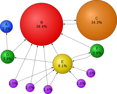
PageRank problem

  • $\mathbf{A} \in \{0,1\}^{n \times n}$ the connectivity matrix of webpages with entries $$ \begin{eqnarray*} a_{ij} = \begin{cases} 1 & \text{if page $i$ links to page $j$} \\ 0 & \text{otherwise} \end{cases}. \end{eqnarray*} $$ $n \approx 10^9$ in May 2017.

  • $r_i = \sum_j a_{ij}$ is the out-degree of page $i$.

  • Larry Page imagines a random surfer wandering on internet according to following rules:

    • From a page $i$ with $r_i>0$
      • with probability $p$, (s)he randomly chooses a link on page $i$ (uniformly) and follows that link to the next page
      • with probability $1-p$, (s)he randomly chooses one page from the set of all $n$ pages (uniformly) and proceeds to that page
    • From a page $i$ with $r_i=0$ (a dangling page), (s)he randomly chooses one page from the set of all $n$ pages (uniformly) and proceeds to that page

The process defines a Markov chain on the space of $n$ pages. Stationary distribution of this Markov chain gives the ranks (probabilities) of each page.

  • Stationary distribution is the top left eigenvector of the transition matrix $\mathbf{P}$ corresponding to eigenvalue 1. Equivalently it can be cast as a linear equation $$ (\mathbf{I} - \mathbf{P}^T) \mathbf{x} = \mathbf{0}. $$

  • Gene Golub: Largest matrix computation in world.

  • GE/LU will take $2 \times (10^9)^3/3/10^{12} \approx 6.66 \times 10^{14}$ seconds $\approx 20$ million years on a tera-flop supercomputer!

  • Iterative methods come to the rescue.

Jacobi method

Solve $\mathbf{A} \mathbf{x} = \mathbf{b}$.

  • Jacobi iteration: $$ x_i^{(t+1)} = \frac{b_i - \sum_{j=1}^{i-1} a_{ij} x_j^{(t)} - \sum_{j=i+1}^n a_{ij} x_j^{(t)}}{a_{ii}}. $$

  • With splitting: $\mathbf{A} = \mathbf{L} + \mathbf{D} + \mathbf{U}$, Jacobi iteration can be written as $$ \mathbf{D} \mathbf{x}^{(t+1)} = - (\mathbf{L} + \mathbf{U}) \mathbf{x}^{(t)} + \mathbf{b}, $$ i.e., $$ \mathbf{x}^{(t+1)} = - \mathbf{D}^{-1} (\mathbf{L} + \mathbf{U}) \mathbf{x}^{(t)} + \mathbf{D}^{-1} \mathbf{b} = - \mathbf{D}^{-1} \mathbf{A} \mathbf{x}^{(t)} + \mathbf{x}^{(t)} + \mathbf{D}^{-1} \mathbf{b}. $$

  • One round costs $2n^2$ flops with an unstructured $\mathbf{A}$. Gain over GE/LU if converges in $o(n)$ iterations. Saving is huge for sparse or structured $\mathbf{A}$. By structured, we mean the matrix-vector multiplication $\mathbf{A} \mathbf{v}$ is fast ($O(n)$ or $O(n \log n)$).

Gauss-Seidel method

  • Gauss-Seidel (GS) iteration: $$ x_i^{(t+1)} = \frac{b_i - \sum_{j=1}^{i-1} a_{ij} x_j^{(t+1)} - \sum_{j=i+1}^n a_{ij} x_j^{(t)}}{a_{ii}}. $$

  • With splitting, $(\mathbf{D} + \mathbf{L}) \mathbf{x}^{(t+1)} = - \mathbf{U} \mathbf{x}^{(t)} + \mathbf{b}$, i.e., $$ \mathbf{x}^{(t+1)} = - (\mathbf{D} + \mathbf{L})^{-1} \mathbf{U} \mathbf{x}^{(t)} + (\mathbf{D} + \mathbf{L})^{-1} \mathbf{b}. $$

  • GS converges for any $\mathbf{x}^{(0)}$ for symmetric and pd $\mathbf{A}$.

  • Convergence rate of Gauss-Seidel is the spectral radius of the $(\mathbf{D} + \mathbf{L})^{-1} \mathbf{U}$.

Successive over-relaxation (SOR)

  • SOR: $$ x_i^{(t+1)} = \omega \left( b_i - \sum_{j=1}^{i-1} a_{ij} x_j^{(t+1)} - \sum_{j=i+1}^n a_{ij} x_j^{(t)} \right) / a_{ii} + (1-\omega) x_i^{(t)}, $$ i.e., $$ \mathbf{x}^{(t+1)} = (\mathbf{D} + \omega \mathbf{L})^{-1} [(1-\omega) \mathbf{D} - \omega \mathbf{U}] \mathbf{x}^{(t)} + (\mathbf{D} + \omega \mathbf{L})^{-1} (\mathbf{D} + \mathbf{L})^{-1} \omega \mathbf{b}. $$

  • Need to pick $\omega \in [0,1]$ beforehand, with the goal of improving convergence rate.

Conjugate gradient method

  • Conjugate gradient and its variants are the top-notch iterative methods for solving huge, structured linear systems.

  • A UCLA invention! Hestenes and Stiefel in 60s.

  • Solving $\mathbf{A} \mathbf{x} = \mathbf{b}$ is equivalent to minimizing the quadratic function $\frac{1}{2} \mathbf{x}^T \mathbf{A} \mathbf{x} - \mathbf{b}^T \mathbf{x}$.

Kershaw's results for a fusion problem.

Method Number of Iterations
Gauss Seidel 208,000
Block SOR methods 765
Incomplete Cholesky conjugate gradient 25

MatrixDepot.jl

MatrixDepot.jl is an extensive collection of test matrices in Julia. After installation, we can check available test matrices by

In [2]:
using MatrixDepot

mdinfo()
┌ Info: verify download of index files...
└ @ MatrixDepot /Users/huazhou/.julia/packages/MatrixDepot/GEDc3/src/MatrixDepot.jl:139
┌ Info: reading database
└ @ MatrixDepot /Users/huazhou/.julia/packages/MatrixDepot/GEDc3/src/download.jl:23
┌ Info: adding metadata...
└ @ MatrixDepot /Users/huazhou/.julia/packages/MatrixDepot/GEDc3/src/download.jl:67
┌ Info: adding svd data...
└ @ MatrixDepot /Users/huazhou/.julia/packages/MatrixDepot/GEDc3/src/download.jl:69
┌ Info: writing database
└ @ MatrixDepot /Users/huazhou/.julia/packages/MatrixDepot/GEDc3/src/download.jl:74
┌ Info: used remote sites are sparse.tamu.edu with MAT index and math.nist.gov with HTML index
└ @ MatrixDepot /Users/huazhou/.julia/packages/MatrixDepot/GEDc3/src/MatrixDepot.jl:141
Out[2]:

Currently loaded Matrices

builtin(#)
1 baart 13 fiedler 25 invhilb 37 parter 49 shaw
2 binomial 14 forsythe 26 invol 38 pascal 50 smallworld
3 blur 15 foxgood 27 kahan 39 pei 51 spikes
4 cauchy 16 frank 28 kms 40 phillips 52 toeplitz
5 chebspec 17 gilbert 29 lehmer 41 poisson 53 tridiag
6 chow 18 golub 30 lotkin 42 prolate 54 triw
7 circul 19 gravity 31 magic 43 randcorr 55 ursell
8 clement 20 grcar 32 minij 44 rando 56 vand
9 companion 21 hadamard 33 moler 45 randsvd 57 wathen
10 deriv2 22 hankel 34 neumann 46 rohess 58 wilkinson
11 dingdong 23 heat 35 oscillate 47 rosser 59 wing
12 erdrey 24 hilb 36 parallax 48 sampling
user(#)
Groups
all local eigen illcond posdef regprob symmetric
builtin user graph inverse random sparse
Suite Sparse of
1 2893
MatrixMarket of
0 498
In [3]:
# List matrices that are positive definite and sparse:
mdlist(:symmetric & :posdef & :sparse)
Out[3]:
2-element Vector{String}:
 "poisson"
 "wathen"
In [4]:
# Get help on Poisson matrix
mdinfo("poisson")
Out[4]:

Poisson Matrix (poisson)

A block tridiagonal matrix from Poisson’s equation. This matrix is sparse, symmetric positive definite and has known eigenvalues. The result is of type SparseMatrixCSC.

Input options:

  • [type,] dim: the dimension of the matirx is dim^2.

Groups: ["inverse", "symmetric", "posdef", "eigen", "sparse"]

References:

G. H. Golub and C. F. Van Loan, Matrix Computations, second edition, Johns Hopkins University Press, Baltimore, Maryland, 1989 (Section 4.5.4).

In [5]:
# Generate a Poisson matrix of dimension n=10
A = matrixdepot("poisson", 10)
Out[5]:
100×100 SparseArrays.SparseMatrixCSC{Float64, Int64} with 460 stored entries:
⠻⣦⡀⠀⠑⢄⠀⠀⠀⠀⠀⠀⠀⠀⠀⠀⠀⠀⠀⠀⠀⠀⠀⠀⠀⠀⠀⠀⠀⠀⠀⠀⠀⠀⠀⠀⠀⠀⠀⠀
⠀⠈⠻⣦⠀⠀⠑⢄⠀⠀⠀⠀⠀⠀⠀⠀⠀⠀⠀⠀⠀⠀⠀⠀⠀⠀⠀⠀⠀⠀⠀⠀⠀⠀⠀⠀⠀⠀⠀⠀
⠑⢄⠀⠀⠻⣦⡀⠀⠑⢄⠀⠀⠀⠀⠀⠀⠀⠀⠀⠀⠀⠀⠀⠀⠀⠀⠀⠀⠀⠀⠀⠀⠀⠀⠀⠀⠀⠀⠀⠀
⠀⠀⠑⢄⠀⠈⠻⣦⠀⠀⠑⢄⠀⠀⠀⠀⠀⠀⠀⠀⠀⠀⠀⠀⠀⠀⠀⠀⠀⠀⠀⠀⠀⠀⠀⠀⠀⠀⠀⠀
⠀⠀⠀⠀⠑⢄⠀⠀⠻⣦⡀⠀⠑⢄⠀⠀⠀⠀⠀⠀⠀⠀⠀⠀⠀⠀⠀⠀⠀⠀⠀⠀⠀⠀⠀⠀⠀⠀⠀⠀
⠀⠀⠀⠀⠀⠀⠑⢄⠀⠈⠻⣦⠀⠀⠑⢄⠀⠀⠀⠀⠀⠀⠀⠀⠀⠀⠀⠀⠀⠀⠀⠀⠀⠀⠀⠀⠀⠀⠀⠀
⠀⠀⠀⠀⠀⠀⠀⠀⠑⢄⠀⠀⠻⣦⡀⠀⠑⢄⠀⠀⠀⠀⠀⠀⠀⠀⠀⠀⠀⠀⠀⠀⠀⠀⠀⠀⠀⠀⠀⠀
⠀⠀⠀⠀⠀⠀⠀⠀⠀⠀⠑⢄⠀⠈⠻⣦⠀⠀⠑⢄⠀⠀⠀⠀⠀⠀⠀⠀⠀⠀⠀⠀⠀⠀⠀⠀⠀⠀⠀⠀
⠀⠀⠀⠀⠀⠀⠀⠀⠀⠀⠀⠀⠑⢄⠀⠀⠻⣦⡀⠀⠱⢄⠀⠀⠀⠀⠀⠀⠀⠀⠀⠀⠀⠀⠀⠀⠀⠀⠀⠀
⠀⠀⠀⠀⠀⠀⠀⠀⠀⠀⠀⠀⠀⠀⠑⢄⠀⠈⠻⣦⠀⠀⠱⢄⠀⠀⠀⠀⠀⠀⠀⠀⠀⠀⠀⠀⠀⠀⠀⠀
⠀⠀⠀⠀⠀⠀⠀⠀⠀⠀⠀⠀⠀⠀⠀⠀⠑⢆⠀⠀⠻⣦⡀⠀⠑⢄⠀⠀⠀⠀⠀⠀⠀⠀⠀⠀⠀⠀⠀⠀
⠀⠀⠀⠀⠀⠀⠀⠀⠀⠀⠀⠀⠀⠀⠀⠀⠀⠀⠑⢆⠀⠈⠻⣦⠀⠀⠑⢄⠀⠀⠀⠀⠀⠀⠀⠀⠀⠀⠀⠀
⠀⠀⠀⠀⠀⠀⠀⠀⠀⠀⠀⠀⠀⠀⠀⠀⠀⠀⠀⠀⠑⢄⠀⠀⠻⣦⡀⠀⠑⢄⠀⠀⠀⠀⠀⠀⠀⠀⠀⠀
⠀⠀⠀⠀⠀⠀⠀⠀⠀⠀⠀⠀⠀⠀⠀⠀⠀⠀⠀⠀⠀⠀⠑⢄⠀⠈⠻⣦⠀⠀⠑⢄⠀⠀⠀⠀⠀⠀⠀⠀
⠀⠀⠀⠀⠀⠀⠀⠀⠀⠀⠀⠀⠀⠀⠀⠀⠀⠀⠀⠀⠀⠀⠀⠀⠑⢄⠀⠀⠻⣦⡀⠀⠑⢄⠀⠀⠀⠀⠀⠀
⠀⠀⠀⠀⠀⠀⠀⠀⠀⠀⠀⠀⠀⠀⠀⠀⠀⠀⠀⠀⠀⠀⠀⠀⠀⠀⠑⢄⠀⠈⠻⣦⠀⠀⠑⢄⠀⠀⠀⠀
⠀⠀⠀⠀⠀⠀⠀⠀⠀⠀⠀⠀⠀⠀⠀⠀⠀⠀⠀⠀⠀⠀⠀⠀⠀⠀⠀⠀⠑⢄⠀⠀⠻⣦⡀⠀⠑⢄⠀⠀
⠀⠀⠀⠀⠀⠀⠀⠀⠀⠀⠀⠀⠀⠀⠀⠀⠀⠀⠀⠀⠀⠀⠀⠀⠀⠀⠀⠀⠀⠀⠑⢄⠀⠈⠻⣦⠀⠀⠑⢄
⠀⠀⠀⠀⠀⠀⠀⠀⠀⠀⠀⠀⠀⠀⠀⠀⠀⠀⠀⠀⠀⠀⠀⠀⠀⠀⠀⠀⠀⠀⠀⠀⠑⢄⠀⠀⠻⣦⡀⠀
⠀⠀⠀⠀⠀⠀⠀⠀⠀⠀⠀⠀⠀⠀⠀⠀⠀⠀⠀⠀⠀⠀⠀⠀⠀⠀⠀⠀⠀⠀⠀⠀⠀⠀⠑⢄⠀⠈⠻⣦
In [6]:
using UnicodePlots
spy(A)
Out[6]:
       ⠀⠀⠀⠀⠀⠀⠀⠀⠀⠀⠀⠀⠀⠀Sparsity Pattern⠀⠀⠀⠀⠀⠀⠀⠀⠀⠀⠀⠀⠀⠀    
       ┌──────────────────────────────────────────┐    
     1 ⠀⠀⠀⠀⠀⠀⠀⠀⠀⠀⠀⠀⠀⠀⠀⠀⠀⠀⠀⠀⠀⠀⠀⠀⠀⠀⠀⠀⠀⠀⠀⠀⠀⠀⠀⠀ > 0
       ⠀⠀⠀⠀⠀⠀⠀⠀⠀⠀⠀⠀⠀⠀⠀⠀⠀⠀⠀⠀⠀⠀⠀⠀⠀⠀⠀⠀⠀⠀⠀⠀⠀⠀ < 0
       ⠀⠀⠀⠀⠀⠀⠀⠀⠀⠀⠀⠀⠀⠀⠀⠀⠀⠀⠀⠀⠀⠀⠀⠀⠀⠀⠀⠀⠀⠀⠀⠀    
       ⠀⠀⠀⠀⠀⠀⠀⠀⠀⠀⠀⠀⠀⠀⠀⠀⠀⠀⠀⠀⠀⠀⠀⠀⠀⠀⠀⠀⠀⠀⠀    
       ⠀⠀⠀⠀⠀⠀⠀⠀⠀⠀⠀⠀⠀⠀⠀⠀⠀⠀⠀⠀⠀⠀⠀⠀⠀⠀⠀⠀⠀⠀⠀    
       ⠀⠀⠀⠀⠀⠀⠀⠀⠀⠀⠀⠀⠀⠀⠀⠀⠀⠀⠀⠀⠀⠀⠀⠀⠀⠀⠀⠀⠀⠀⠀⠀    
       ⠀⠀⠀⠀⠀⠀⠀⠀⠀⠀⠀⠀⠀⠀⠀⠀⠀⠀⠀⠀⠀⠀⠀⠀⠀⠀⠀⠀⠀⠀⠀    
       ⠀⠀⠀⠀⠀⠀⠀⠀⠀⠀⠀⠀⠀⠀⠀⠀⠀⠀⠀⠀⠀⠀⠀⠀⠀⠀⠀⠀⠀⠀⠀    
       ⠀⠀⠀⠀⠀⠀⠀⠀⠀⠀⠀⠀⠀⠀⠀⠀⠀⠀⠀⠀⠀⠀⠀⠀⠀⠀⠀⠀⠀⠀⠀    
       ⠀⠀⠀⠀⠀⠀⠀⠀⠀⠀⠀⠀⠀⠀⠀⠀⠀⠀⠀⠀⠀⠀⠀⠀⠀⠀⠀⠀⠀⠀⠀    
       ⠀⠀⠀⠀⠀⠀⠀⠀⠀⠀⠀⠀⠀⠀⠀⠀⠀⠀⠀⠀⠀⠀⠀⠀⠀⠀⠀⠀⠀⠀⠀⠀    
       ⠀⠀⠀⠀⠀⠀⠀⠀⠀⠀⠀⠀⠀⠀⠀⠀⠀⠀⠀⠀⠀⠀⠀⠀⠀⠀⠀⠀⠀⠀⠀    
       ⠀⠀⠀⠀⠀⠀⠀⠀⠀⠀⠀⠀⠀⠀⠀⠀⠀⠀⠀⠀⠀⠀⠀⠀⠀⠀⠀⠀⠀⠀⠀    
       ⠀⠀⠀⠀⠀⠀⠀⠀⠀⠀⠀⠀⠀⠀⠀⠀⠀⠀⠀⠀⠀⠀⠀⠀⠀⠀⠀⠀⠀⠀⠀    
       ⠀⠀⠀⠀⠀⠀⠀⠀⠀⠀⠀⠀⠀⠀⠀⠀⠀⠀⠀⠀⠀⠀⠀⠀⠀⠀⠀⠀⠀⠀⠀    
       ⠀⠀⠀⠀⠀⠀⠀⠀⠀⠀⠀⠀⠀⠀⠀⠀⠀⠀⠀⠀⠀⠀⠀⠀⠀⠀⠀⠀⠀⠀⠀⠀    
       ⠀⠀⠀⠀⠀⠀⠀⠀⠀⠀⠀⠀⠀⠀⠀⠀⠀⠀⠀⠀⠀⠀⠀⠀⠀⠀⠀⠀⠀⠀⠀    
       ⠀⠀⠀⠀⠀⠀⠀⠀⠀⠀⠀⠀⠀⠀⠀⠀⠀⠀⠀⠀⠀⠀⠀⠀⠀⠀⠀⠀⠀⠀⠀    
       ⠀⠀⠀⠀⠀⠀⠀⠀⠀⠀⠀⠀⠀⠀⠀⠀⠀⠀⠀⠀⠀⠀⠀⠀⠀⠀⠀⠀⠀⠀⠀⠀    
       ⠀⠀⠀⠀⠀⠀⠀⠀⠀⠀⠀⠀⠀⠀⠀⠀⠀⠀⠀⠀⠀⠀⠀⠀⠀⠀⠀⠀⠀⠀⠀⠀⠀⠀    
   100 ⠀⠀⠀⠀⠀⠀⠀⠀⠀⠀⠀⠀⠀⠀⠀⠀⠀⠀⠀⠀⠀⠀⠀⠀⠀⠀⠀⠀⠀⠀⠀⠀⠀⠀⠀⠀    
       └──────────────────────────────────────────┘1⠀⠀⠀⠀⠀⠀⠀⠀⠀⠀⠀⠀⠀⠀⠀⠀⠀⠀⠀⠀⠀⠀⠀⠀⠀⠀⠀⠀⠀⠀⠀⠀⠀⠀⠀⠀⠀⠀100⠀    
       ⠀⠀⠀⠀⠀⠀⠀⠀⠀⠀⠀⠀⠀⠀⠀⠀460 nonzeros⠀⠀⠀⠀⠀⠀⠀⠀⠀⠀⠀⠀⠀⠀⠀⠀    
In [7]:
# Get help on Wathen matrix
mdinfo("wathen")
Out[7]:

Wathen Matrix (wathen)

Wathen Matrix is a sparse, symmetric positive, random matrix arose from the finite element method. The generated matrix is the consistent mass matrix for a regular nx-by-ny grid of 8-nodes.

Input options:

  • [type,] nx, ny: the dimension of the matrix is equal to 3 * nx * ny + 2 * nx * ny + 1.
  • [type,] n: nx = ny = n.

Groups: ["symmetric", "posdef", "eigen", "random", "sparse"]

References:

A. J. Wathen, Realistic eigenvalue bounds for the Galerkin mass matrix, IMA J. Numer. Anal., 7 (1987), pp. 449-457.

In [8]:
# Generate a Wathen matrix of dimension n=5
A = matrixdepot("wathen", 5)
Out[8]:
96×96 SparseArrays.SparseMatrixCSC{Float64, Int64} with 1256 stored entries:
⠿⣧⣀⠀⠸⣧⡀⠿⣧⣀⠀⠀⠀⠀⠀⠀⠀⠀⠀⠀⠀⠀⠀⠀⠀⠀⠀⠀⠀⠀⠀⠀⠀⠀⠀⠀⠀⠀⠀⠀
⠀⠘⢻⣶⡀⠘⣇⠀⠘⢻⣶⡀⠀⠀⠀⠀⠀⠀⠀⠀⠀⠀⠀⠀⠀⠀⠀⠀⠀⠀⠀⠀⠀⠀⠀⠀⠀⠀⠀⠀
⠶⣦⣀⠈⠱⣦⡉⠶⣦⣀⠈⠁⠀⠀⠀⠀⠀⠀⠀⠀⠀⠀⠀⠀⠀⠀⠀⠀⠀⠀⠀⠀⠀⠀⠀⠀⠀⠀⠀⠀
⣤⡌⠉⠙⢣⡌⠛⣤⡌⠉⠙⢣⡄⠀⣤⡄⠀⠀⠀⠀⠀⠀⠀⠀⠀⠀⠀⠀⠀⠀⠀⠀⠀⠀⠀⠀⠀⠀⠀⠀
⠉⢻⣶⣀⠈⢻⡆⠉⢻⣶⣀⠈⢻⣆⠉⠛⣷⣀⠀⠀⠀⠀⠀⠀⠀⠀⠀⠀⠀⠀⠀⠀⠀⠀⠀⠀⠀⠀⠀⠀
⠀⠀⠘⠻⠆⠀⠷⣀⡀⠘⠻⢆⡀⠻⣀⡀⠘⠻⠶⠀⠀⠀⠀⠀⠀⠀⠀⠀⠀⠀⠀⠀⠀⠀⠀⠀⠀⠀⠀⠀
⠀⠀⠀⠀⠀⠀⠀⠉⠻⢶⣤⡈⠻⣦⠉⠛⢷⣤⣀⠀⠀⠀⠀⠀⠀⠀⠀⠀⠀⠀⠀⠀⠀⠀⠀⠀⠀⠀⠀⠀
⠀⠀⠀⠀⠀⠀⠀⠿⣧⠀⠀⠸⣧⠀⠿⣧⡄⠀⠸⣧⠀⠿⣧⡄⠀⠀⠀⠀⠀⠀⠀⠀⠀⠀⠀⠀⠀⠀⠀⠀
⠀⠀⠀⠀⠀⠀⠀⠀⠙⢻⣶⡀⠙⣷⠀⠉⢻⣶⣀⠙⣷⡀⠉⢻⣶⣀⠀⠀⠀⠀⠀⠀⠀⠀⠀⠀⠀⠀⠀⠀
⠀⠀⠀⠀⠀⠀⠀⠀⠀⠀⠘⠃⠀⠘⠶⣦⣄⠘⠻⣦⡘⠷⣦⣄⠘⠛⠀⠀⠀⠀⠀⠀⠀⠀⠀⠀⠀⠀⠀⠀
⠀⠀⠀⠀⠀⠀⠀⠀⠀⠀⠀⠀⠀⠀⣤⡄⠙⠻⢶⡌⠻⣦⡄⠙⠻⠶⡄⠀⢠⡄⠀⠀⠀⠀⠀⠀⠀⠀⠀⠀
⠀⠀⠀⠀⠀⠀⠀⠀⠀⠀⠀⠀⠀⠀⠉⠿⣧⣀⠈⢿⣄⠉⠿⣧⣀⠀⢿⣄⠈⠿⣧⣄⠀⠀⠀⠀⠀⠀⠀⠀
⠀⠀⠀⠀⠀⠀⠀⠀⠀⠀⠀⠀⠀⠀⠀⠀⠘⢻⣶⠀⢻⡆⠀⠘⢻⣶⠀⢻⡆⠀⠀⢻⣶⠀⠀⠀⠀⠀⠀⠀
⠀⠀⠀⠀⠀⠀⠀⠀⠀⠀⠀⠀⠀⠀⠀⠀⠀⠀⠀⠀⠀⠉⠛⢷⣤⣀⠻⣦⡈⠛⠷⣦⣀⠀⠀⠀⠀⠀⠀⠀
⠀⠀⠀⠀⠀⠀⠀⠀⠀⠀⠀⠀⠀⠀⠀⠀⠀⠀⠀⠀⠀⠶⣦⡄⠈⠉⣦⠈⠱⣦⡄⠈⠉⢶⠀⠰⣦⡄⠀⠀
⠀⠀⠀⠀⠀⠀⠀⠀⠀⠀⠀⠀⠀⠀⠀⠀⠀⠀⠀⠀⠀⠀⠉⢿⣤⣀⠹⣧⡀⠉⠿⣧⣀⠸⣧⡀⠉⠿⣧⣀
⠀⠀⠀⠀⠀⠀⠀⠀⠀⠀⠀⠀⠀⠀⠀⠀⠀⠀⠀⠀⠀⠀⠀⠀⠘⠛⠀⠘⢣⣄⣀⡘⠛⣤⡘⢣⣄⣀⡘⠛
⠀⠀⠀⠀⠀⠀⠀⠀⠀⠀⠀⠀⠀⠀⠀⠀⠀⠀⠀⠀⠀⠀⠀⠀⠀⠀⠀⠀⢀⡀⠉⠻⠶⣈⠻⢆⡀⠉⠻⠶
⠀⠀⠀⠀⠀⠀⠀⠀⠀⠀⠀⠀⠀⠀⠀⠀⠀⠀⠀⠀⠀⠀⠀⠀⠀⠀⠀⠀⠈⠿⣧⡄⠀⢹⡄⠈⠿⣧⡄⠀
⠀⠀⠀⠀⠀⠀⠀⠀⠀⠀⠀⠀⠀⠀⠀⠀⠀⠀⠀⠀⠀⠀⠀⠀⠀⠀⠀⠀⠀⠀⠉⢻⣶⠈⢻⡆⠀⠉⢻⣶
In [9]:
spy(A)
Out[9]:
      ⠀⠀⠀⠀⠀⠀⠀⠀⠀⠀⠀⠀⠀⠀Sparsity Pattern⠀⠀⠀⠀⠀⠀⠀⠀⠀⠀⠀⠀⠀⠀    
      ┌──────────────────────────────────────────┐    
    1 ⠀⠀⠀⠀⠀⠀⠀⠀⠀⠀⠀⠀⠀⠀⠀⠀⠀⠀⠀⠀⠀⠀⠀⠀⠀⠀⠀⠀⠀⠀⠀⠀⠀⠀ > 0
      ⠀⠀⠀⠀⠀⠀⠀⠀⠀⠀⠀⠀⠀⠀⠀⠀⠀⠀⠀⠀⠀⠀⠀⠀⠀⠀⠀⠀⠀ < 0
      ⠀⠀⠀⠀⠀⠀⠀⠀⠀⠀⠀⠀⠀⠀⠀⠀⠀⠀⠀⠀⠀⠀⠀⠀⠀⠀⠀⠀⠀    
      ⠀⠀⠀⠀⠀⠀⠀⠀⠀⠀⠀⠀⠀⠀⠀⠀⠀⠀⠀⠀⠀⠀⠀⠀⠀⠀⠀    
      ⠀⠀⠀⠀⠀⠀⠀⠀⠀⠀⠀⠀⠀⠀⠀⠀⠀⠀⠀⠀⠀⠀⠀⠀    
      ⠀⠀⠀⠀⠀⠀⠀⠀⠀⠀⠀⠀⠀⠀⠀⠀⠀⠀⠀⠀⠀⠀⠀⠀    
      ⠀⠀⠀⠀⠀⠀⠀⠀⠀⠀⠀⠀⠀⠀⠀⠀⠀⠀⠀⠀⠀⠀⠀⠀⠀    
      ⠀⠀⠀⠀⠀⠀⠀⠀⠀⠀⠀⠀⠀⠀⠀⠀⠀⠀⠀⠀⠀⠀⠀⠀⠀    
      ⠀⠀⠀⠀⠀⠀⠀⠀⠀⠀⠀⠀⠀⠀⠀⠀⠀⠀⠀⠀⠀⠀⠀    
      ⠀⠀⠀⠀⠀⠀⠀⠀⠀⠀⠀⠀⠀⠀⠀⠀⠀⠀⠀⠀⠀⠀⠀⠀⠀    
      ⠀⠀⠀⠀⠀⠀⠀⠀⠀⠀⠀⠀⠀⠀⠀⠀⠀⠀⠀⠀⠀⠀⠀⠀⠀⠀⠀⠀⠀⠀    
      ⠀⠀⠀⠀⠀⠀⠀⠀⠀⠀⠀⠀⠀⠀⠀⠀⠀⠀⠀⠀⠀⠀⠀⠀⠀    
      ⠀⠀⠀⠀⠀⠀⠀⠀⠀⠀⠀⠀⠀⠀⠀⠀⠀⠀⠀⠀⠀⠀⠀    
      ⠀⠀⠀⠀⠀⠀⠀⠀⠀⠀⠀⠀⠀⠀⠀⠀⠀⠀⠀⠀⠀⠀⠀⠀⠀    
      ⠀⠀⠀⠀⠀⠀⠀⠀⠀⠀⠀⠀⠀⠀⠀⠀⠀⠀⠀⠀⠀⠀⠀⠀⠀    
      ⠀⠀⠀⠀⠀⠀⠀⠀⠀⠀⠀⠀⠀⠀⠀⠀⠀⠀⠀⠀⠀⠀⠀⠀    
      ⠀⠀⠀⠀⠀⠀⠀⠀⠀⠀⠀⠀⠀⠀⠀⠀⠀⠀⠀⠀⠀⠀⠀⠀    
      ⠀⠀⠀⠀⠀⠀⠀⠀⠀⠀⠀⠀⠀⠀⠀⠀⠀⠀⠀⠀⠀⠀⠀⠀⠀⠀⠀    
      ⠀⠀⠀⠀⠀⠀⠀⠀⠀⠀⠀⠀⠀⠀⠀⠀⠀⠀⠀⠀⠀⠀⠀⠀⠀⠀⠀⠀⠀    
      ⠀⠀⠀⠀⠀⠀⠀⠀⠀⠀⠀⠀⠀⠀⠀⠀⠀⠀⠀⠀⠀⠀⠀⠀⠀⠀⠀⠀⠀    
   96 ⠀⠀⠀⠀⠀⠀⠀⠀⠀⠀⠀⠀⠀⠀⠀⠀⠀⠀⠀⠀⠀⠀⠀⠀⠀⠀⠀⠀⠀⠀⠀⠀⠀⠀    
      └──────────────────────────────────────────┘1⠀⠀⠀⠀⠀⠀⠀⠀⠀⠀⠀⠀⠀⠀⠀⠀⠀⠀⠀⠀⠀⠀⠀⠀⠀⠀⠀⠀⠀⠀⠀⠀⠀⠀⠀⠀⠀⠀⠀96⠀    
      ⠀⠀⠀⠀⠀⠀⠀⠀⠀⠀⠀⠀⠀⠀⠀⠀1256 nonzeros⠀⠀⠀⠀⠀⠀⠀⠀⠀⠀⠀⠀⠀⠀⠀    

Numerical examples

The IterativeSolvers.jl package implements most commonly used iterative solvers.

Generate test matrix

In [10]:
using BenchmarkTools, IterativeSolvers, LinearAlgebra, MatrixDepot, Random

Random.seed!(280)

n = 100
# Poisson matrix of dimension n^2=10000, pd and sparse
A = matrixdepot("poisson", n)
@show typeof(A)
# dense matrix representation of A
Afull = convert(Matrix, A)
@show typeof(Afull)
# sparsity level
count(!iszero, A) / length(A)
typeof(A) = SparseArrays.SparseMatrixCSC{Float64, Int64}
typeof(Afull) = Matrix{Float64}
Out[10]:
0.000496
In [11]:
spy(A)
Out[11]:
         ⠀⠀⠀⠀⠀⠀⠀⠀⠀⠀⠀⠀⠀⠀Sparsity Pattern⠀⠀⠀⠀⠀⠀⠀⠀⠀⠀⠀⠀⠀⠀    
         ┌──────────────────────────────────────────┐    
       1 ⠀⠀⠀⠀⠀⠀⠀⠀⠀⠀⠀⠀⠀⠀⠀⠀⠀⠀⠀⠀⠀⠀⠀⠀⠀⠀⠀⠀⠀⠀⠀⠀⠀⠀⠀⠀⠀⠀⠀ > 0
         ⠀⠀⠀⠀⠀⠀⠀⠀⠀⠀⠀⠀⠀⠀⠀⠀⠀⠀⠀⠀⠀⠀⠀⠀⠀⠀⠀⠀⠀⠀⠀⠀⠀⠀⠀⠀⠀ < 0
         ⠀⠀⠀⠀⠀⠀⠀⠀⠀⠀⠀⠀⠀⠀⠀⠀⠀⠀⠀⠀⠀⠀⠀⠀⠀⠀⠀⠀⠀⠀⠀⠀⠀⠀⠀⠀⠀⠀    
         ⠀⠀⠀⠀⠀⠀⠀⠀⠀⠀⠀⠀⠀⠀⠀⠀⠀⠀⠀⠀⠀⠀⠀⠀⠀⠀⠀⠀⠀⠀⠀⠀⠀⠀⠀⠀⠀⠀    
         ⠀⠀⠀⠀⠀⠀⠀⠀⠀⠀⠀⠀⠀⠀⠀⠀⠀⠀⠀⠀⠀⠀⠀⠀⠀⠀⠀⠀⠀⠀⠀⠀⠀⠀⠀⠀⠀⠀    
         ⠀⠀⠀⠀⠀⠀⠀⠀⠀⠀⠀⠀⠀⠀⠀⠀⠀⠀⠀⠀⠀⠀⠀⠀⠀⠀⠀⠀⠀⠀⠀⠀⠀⠀⠀⠀⠀⠀    
         ⠀⠀⠀⠀⠀⠀⠀⠀⠀⠀⠀⠀⠀⠀⠀⠀⠀⠀⠀⠀⠀⠀⠀⠀⠀⠀⠀⠀⠀⠀⠀⠀⠀⠀⠀⠀⠀⠀    
         ⠀⠀⠀⠀⠀⠀⠀⠀⠀⠀⠀⠀⠀⠀⠀⠀⠀⠀⠀⠀⠀⠀⠀⠀⠀⠀⠀⠀⠀⠀⠀⠀⠀⠀⠀⠀⠀⠀    
         ⠀⠀⠀⠀⠀⠀⠀⠀⠀⠀⠀⠀⠀⠀⠀⠀⠀⠀⠀⠀⠀⠀⠀⠀⠀⠀⠀⠀⠀⠀⠀⠀⠀⠀⠀⠀⠀⠀    
         ⠀⠀⠀⠀⠀⠀⠀⠀⠀⠀⠀⠀⠀⠀⠀⠀⠀⠀⠀⠀⠀⠀⠀⠀⠀⠀⠀⠀⠀⠀⠀⠀⠀⠀⠀⠀⠀⠀    
         ⠀⠀⠀⠀⠀⠀⠀⠀⠀⠀⠀⠀⠀⠀⠀⠀⠀⠀⠀⠀⠀⠀⠀⠀⠀⠀⠀⠀⠀⠀⠀⠀⠀⠀⠀⠀⠀⠀    
         ⠀⠀⠀⠀⠀⠀⠀⠀⠀⠀⠀⠀⠀⠀⠀⠀⠀⠀⠀⠀⠀⠀⠀⠀⠀⠀⠀⠀⠀⠀⠀⠀⠀⠀⠀⠀⠀⠀    
         ⠀⠀⠀⠀⠀⠀⠀⠀⠀⠀⠀⠀⠀⠀⠀⠀⠀⠀⠀⠀⠀⠀⠀⠀⠀⠀⠀⠀⠀⠀⠀⠀⠀⠀⠀⠀⠀⠀    
         ⠀⠀⠀⠀⠀⠀⠀⠀⠀⠀⠀⠀⠀⠀⠀⠀⠀⠀⠀⠀⠀⠀⠀⠀⠀⠀⠀⠀⠀⠀⠀⠀⠀⠀⠀⠀⠀⠀    
         ⠀⠀⠀⠀⠀⠀⠀⠀⠀⠀⠀⠀⠀⠀⠀⠀⠀⠀⠀⠀⠀⠀⠀⠀⠀⠀⠀⠀⠀⠀⠀⠀⠀⠀⠀⠀⠀⠀    
         ⠀⠀⠀⠀⠀⠀⠀⠀⠀⠀⠀⠀⠀⠀⠀⠀⠀⠀⠀⠀⠀⠀⠀⠀⠀⠀⠀⠀⠀⠀⠀⠀⠀⠀⠀⠀⠀⠀    
         ⠀⠀⠀⠀⠀⠀⠀⠀⠀⠀⠀⠀⠀⠀⠀⠀⠀⠀⠀⠀⠀⠀⠀⠀⠀⠀⠀⠀⠀⠀⠀⠀⠀⠀⠀⠀⠀⠀    
         ⠀⠀⠀⠀⠀⠀⠀⠀⠀⠀⠀⠀⠀⠀⠀⠀⠀⠀⠀⠀⠀⠀⠀⠀⠀⠀⠀⠀⠀⠀⠀⠀⠀⠀⠀⠀⠀⠀    
         ⠀⠀⠀⠀⠀⠀⠀⠀⠀⠀⠀⠀⠀⠀⠀⠀⠀⠀⠀⠀⠀⠀⠀⠀⠀⠀⠀⠀⠀⠀⠀⠀⠀⠀⠀⠀⠀⠀    
         ⠀⠀⠀⠀⠀⠀⠀⠀⠀⠀⠀⠀⠀⠀⠀⠀⠀⠀⠀⠀⠀⠀⠀⠀⠀⠀⠀⠀⠀⠀⠀⠀⠀⠀⠀⠀⠀    
   10000 ⠀⠀⠀⠀⠀⠀⠀⠀⠀⠀⠀⠀⠀⠀⠀⠀⠀⠀⠀⠀⠀⠀⠀⠀⠀⠀⠀⠀⠀⠀⠀⠀⠀⠀⠀⠀⠀⠀⠀    
         └──────────────────────────────────────────┘1⠀⠀⠀⠀⠀⠀⠀⠀⠀⠀⠀⠀⠀⠀⠀⠀⠀⠀⠀⠀⠀⠀⠀⠀⠀⠀⠀⠀⠀⠀⠀⠀⠀⠀⠀⠀10000⠀    
         ⠀⠀⠀⠀⠀⠀⠀⠀⠀⠀⠀⠀⠀⠀⠀49600 nonzeros⠀⠀⠀⠀⠀⠀⠀⠀⠀⠀⠀⠀⠀⠀⠀    
In [12]:
# storage difference
Base.summarysize(A), Base.summarysize(Afull)
Out[12]:
(873768, 800000040)

Matrix-vector muliplication

In [13]:
# randomly generated vector of length n^2
b = randn(n^2)
# dense matrix-vector multiplication
@benchmark $Afull * $b
Out[13]:
BenchmarkTools.Trial: 108 samples with 1 evaluation.
 Range (minmax):  37.348 ms53.127 ms   GC (min … max): 0.00% … 0.00%
 Time  (median):     47.148 ms               GC (median):    0.00%
 Time  (mean ± σ):   46.548 ms ±  3.533 ms   GC (mean ± σ):  0.00% ± 0.00%

              ▂▂▂ ▂       ▂▂    ▂     ▅    █ █▂▂▅ ▂  ▅▂█▅ ▅  
  ▅▁▁▁▁▁▁▁▁▁▁▁███▅█▅▅▅▅▁████▅▅█▅█▅███▅█▁▁██▅████▅█▅▁████▅█ ▅
  37.3 ms         Histogram: frequency by time        51.7 ms <

 Memory estimate: 78.17 KiB, allocs estimate: 2.
In [14]:
# sparse matrix-vector multiplication
@benchmark $A * $b
Out[14]:
BenchmarkTools.Trial: 10000 samples with 1 evaluation.
 Range (minmax):  66.407 μs 53.323 ms   GC (min … max): 0.00% … 99.71%
 Time  (median):     86.076 μs                GC (median):    0.00%
 Time  (mean ± σ):   95.826 μs ± 532.564 μs   GC (mean ± σ):  5.55% ±  1.00%

         ▇██▇▆▅▅▃▃▂▂▂▁▃▃▂▁▁▁                                 ▃
  ▅▃▅▃▄▅▅████████████████████████▇▇▇▇▆▅▇▆▇▆▅▆▆▅▅▅▅▃▅▁▅▄▃▄▃▅▇ █
  66.4 μs       Histogram: log(frequency) by time       181 μs <

 Memory estimate: 78.17 KiB, allocs estimate: 2.

Dense solve via Cholesky

In [15]:
# record the Cholesky solution
xchol = cholesky(Afull) \ b;
In [16]:
# dense solve via Cholesky
@benchmark cholesky($Afull) \ $b
Out[16]:
BenchmarkTools.Trial: 2 samples with 1 evaluation.
 Range (minmax):  3.211 s  3.278 s   GC (min … max): 1.28% … 0.01%
 Time  (median):     3.245 s               GC (median):    0.64%
 Time  (mean ± σ):   3.245 s ± 47.453 ms   GC (mean ± σ):  0.64% ± 0.89%

                              ▁▁▁▁▁▁▁▁▁▁▁▁▁▁▁▁▁▁▁▁▁▁▁▁▁▁▁▁▁▁▁▁▁▁▁▁▁▁▁▁▁▁▁▁▁▁▁▁▁▁▁▁▁▁█ ▁
  3.21 s         Histogram: frequency by time        3.28 s <

 Memory estimate: 763.02 MiB, allocs estimate: 6.

Jacobi solver

It seems that Jacobi solver doesn't give the correct answer.

In [17]:
xjacobi = jacobi(A, b)
@show norm(xjacobi - xchol)
norm(xjacobi - xchol) = 498.7144076230417
Out[17]:
498.7144076230417

Reading documentation we found that the default value of maxiter is 10. A couple trial runs shows that 30000 Jacobi iterations are enough to get an accurate solution.

In [18]:
xjacobi = jacobi(A, b, maxiter=30000)
@show norm(xjacobi - xchol)
norm(xjacobi - xchol) = 1.626836219074868e-5
Out[18]:
1.626836219074868e-5
In [19]:
@benchmark jacobi($A, $b, maxiter=30000)
Out[19]:
BenchmarkTools.Trial: 3 samples with 1 evaluation.
 Range (minmax):  2.240 s  2.325 s   GC (min … max): 0.00% … 0.00%
 Time  (median):     2.253 s               GC (median):    0.00%
 Time  (mean ± σ):   2.273 s ± 45.880 ms   GC (mean ± σ):  0.00% ± 0.00%

   ▁▁▁▁▁▁▁█▁▁▁▁▁▁▁▁▁▁▁▁▁▁▁▁▁▁▁▁▁▁▁▁▁▁▁▁▁▁▁▁▁▁▁▁▁▁▁▁▁▁▁▁▁▁█ ▁
  2.24 s         Histogram: frequency by time        2.33 s <

 Memory estimate: 2.06 MiB, allocs estimate: 30008.

Gauss-Seidal

In [20]:
# Gauss-Seidel solution is fairly close to Cholesky solution after 15000 iters
xgs = gauss_seidel(A, b, maxiter=15000)
@show norm(xgs - xchol)
norm(xgs - xchol) = 1.429290496951622e-5
Out[20]:
1.429290496951622e-5
In [21]:
@benchmark gauss_seidel($A, $b, maxiter=15000)
Out[21]:
BenchmarkTools.Trial: 3 samples with 1 evaluation.
 Range (minmax):  1.837 s  1.867 s   GC (min … max): 0.00% … 0.00%
 Time  (median):     1.843 s               GC (median):    0.00%
 Time  (mean ± σ):   1.849 s ± 15.648 ms   GC (mean ± σ):  0.00% ± 0.00%

   ▁▁▁▁▁▁▁▁▁▁█▁▁▁▁▁▁▁▁▁▁▁▁▁▁▁▁▁▁▁▁▁▁▁▁▁▁▁▁▁▁▁▁▁▁▁▁▁▁▁▁▁▁▁█ ▁
  1.84 s         Histogram: frequency by time        1.87 s <

 Memory estimate: 156.58 KiB, allocs estimate: 7.

SOR

In [22]:
# symmetric SOR with ω=0.75
xsor = ssor(A, b, 0.75, maxiter=10000)
@show norm(xsor - xchol)
norm(xsor - xchol) = 0.0002980091296489782
Out[22]:
0.0002980091296489782
In [23]:
@benchmark sor($A, $b, 0.75, maxiter=10000)
Out[23]:
BenchmarkTools.Trial: 4 samples with 1 evaluation.
 Range (minmax):  1.426 s 1.446 s   GC (min … max): 0.00% … 0.00%
 Time  (median):     1.438 s              GC (median):    0.00%
 Time  (mean ± σ):   1.437 s ± 9.470 ms   GC (mean ± σ):  0.00% ± 0.00%

  █              █                                  █    █  
  █▁▁▁▁▁▁▁▁▁▁▁▁▁▁█▁▁▁▁▁▁▁▁▁▁▁▁▁▁▁▁▁▁▁▁▁▁▁▁▁▁▁▁▁▁▁▁█▁▁▁▁█ ▁
  1.43 s        Histogram: frequency by time        1.45 s <

 Memory estimate: 547.27 KiB, allocs estimate: 20009.

Conjugate Gradient

In [24]:
# conjugate gradient
xcg = cg(A, b)
@show norm(xcg - xchol)
norm(xcg - xchol) = 1.2232567404794239e-5
Out[24]:
1.2232567404794239e-5
In [25]:
@benchmark cg($A, $b)
Out[25]:
BenchmarkTools.Trial: 228 samples with 1 evaluation.
 Range (minmax):  20.099 ms36.722 ms   GC (min … max): 0.00% … 0.00%
 Time  (median):     21.165 ms               GC (median):    0.00%
 Time  (mean ± σ):   21.988 ms ±  2.768 ms   GC (mean ± σ):  0.00% ± 0.00%

    ██                                                     
  ▃████▆▆▄▃▃▃▂▃▂▁▁▁▁▁▂▁▁▁▁▁▂▁▁▁▁▁▁▁▁▁▁▁▃▂▂▁▁▂▁▁▁▂▁▃▁▁▂▂▁▁▁▂ ▃
  20.1 ms         Histogram: frequency by time        34.5 ms <

 Memory estimate: 313.39 KiB, allocs estimate: 16.