GPU Computing in Julia¶

This session introduces GPU computing in Julia.

GPGPU¶

GPUs are ubiquitous in modern computers. Following are GPUs today's typical computer systems.

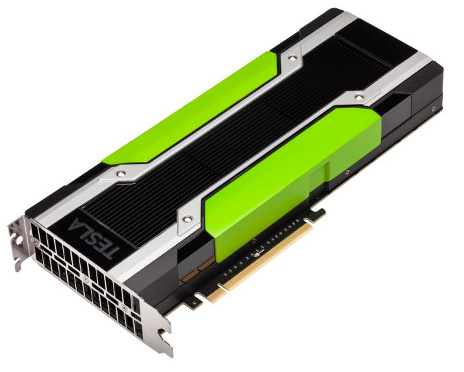
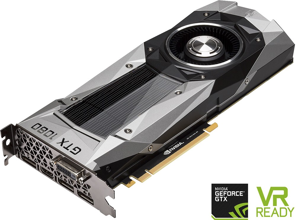
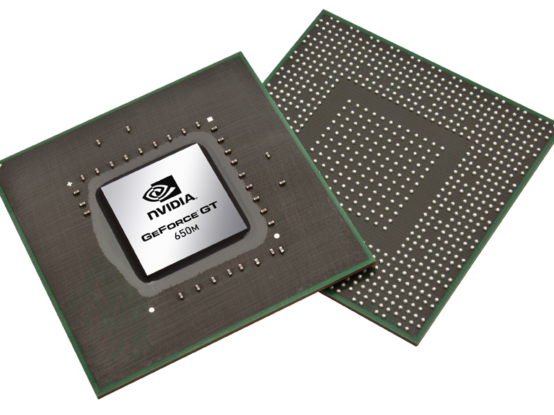
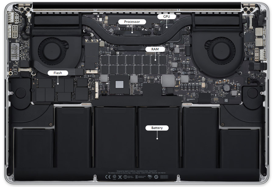
NVIDIA GPUs	Tesla K80	GTX 1080	GT 650M

Computers	servers, cluster	desktop	laptop

Main usage	scientific computing	daily work, gaming	daily work
Memory	24 GB	8 GB	1GB
Memory bandwidth	480 GB/sec	320 GB/sec	80GB/sec
Number of cores	4992	2560	384
Processor clock	562 MHz	1.6 GHz	0.9GHz
Peak DP performance	2.91 TFLOPS	257 GFLOPS
Peak SP performance	8.73 TFLOPS	8228 GFLOPS	691Gflops

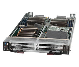
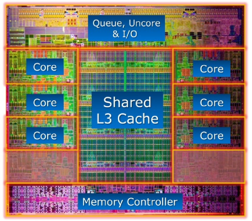
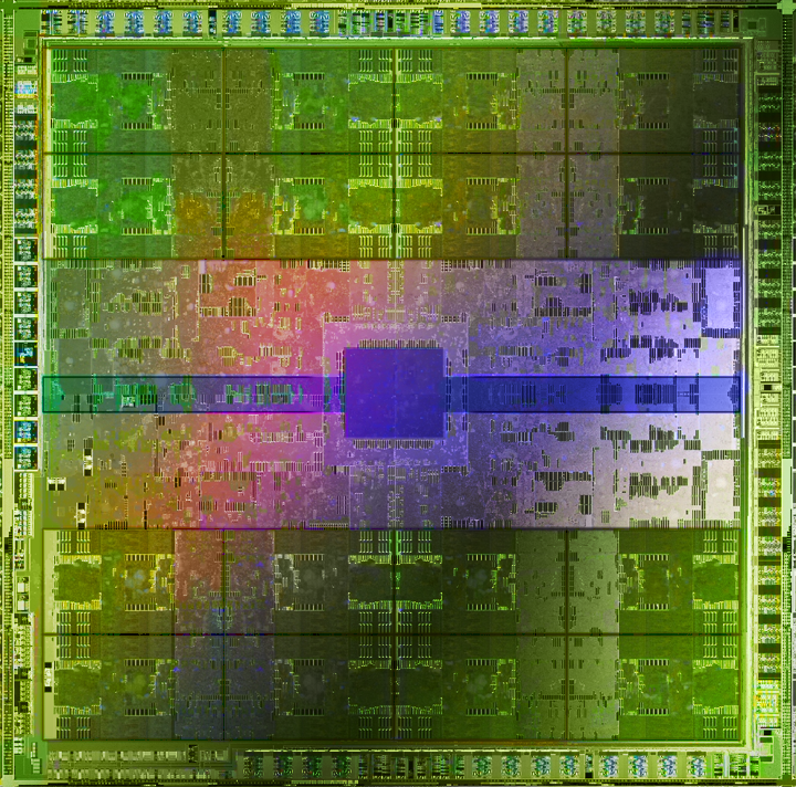
GPU architecture vs CPU architecture.

GPUs contain 100s of processing cores on a single card; several cards can fit in a desktop PC
Each core carries out the same operations in parallel on different input data -- single program, multiple data (SPMD) paradigm
Extremely high arithmetic intensity if one can transfer the data onto and results off of the processors quickly

GPGPU in Julia¶

GPU support by Julia is under active development. Check JuliaGPU for currently available packages.

There are at least two paradigms to program GPU in Julia.

CUDA is an ecosystem exclusively for Nvidia GPUs. There are extensive CUDA libraries for scientific computing: CuBLAS, CuRAND, CuSparse, CuSolve, CuDNN, ...

The CUDA.jl package allows defining arrays on Nvidia GPUs and overloads many common operations.
The AMDGPU.jl package allows defining arrays on AMD GPUs and overloads many common operations.
Warning: Most recent Apple operating system iOS 10.15 (Catalina) does not support CUDA yet.

I'll illustrate using CuArrays on my Linux box running CentOS 7. It has a NVIDIA GeForce RTX 2080 Ti OC with 11GB GDDR6 (14 Gbps) and 4352 cores.

versioninfo()

Julia Version 1.7.2
Commit bf53498635 (2022-02-06 15:21 UTC)
Platform Info:
  OS: Linux (x86_64-pc-linux-gnu)
  CPU: Intel(R) Core(TM) i9-9920X CPU @ 3.50GHz
  WORD_SIZE: 64
  LIBM: libopenlibm
  LLVM: libLLVM-12.0.1 (ORCJIT, skylake-avx512)
Environment:
  JULIA_NUM_THREADS = 8

Query GPU devices in the system¶

using CUDA

CUDA.versioninfo()

CUDA toolkit 11.6, artifact installation
NVIDIA driver 470.57.2, for CUDA 11.4
CUDA driver 11.4

Libraries: 
- CUBLAS: 11.8.1
- CURAND: 10.2.9
- CUFFT: 10.7.0
- CUSOLVER: 11.3.2
- CUSPARSE: 11.7.1
- CUPTI: 16.0.0
- NVML: 11.0.0+470.57.2
- CUDNN: 8.30.2 (for CUDA 11.5.0)
- CUTENSOR: 1.4.0 (for CUDA 11.5.0)

Toolchain:
- Julia: 1.7.2
- LLVM: 12.0.1
- PTX ISA support: 3.2, 4.0, 4.1, 4.2, 4.3, 5.0, 6.0, 6.1, 6.3, 6.4, 6.5, 7.0
- Device capability support: sm_35, sm_37, sm_50, sm_52, sm_53, sm_60, sm_61, sm_62, sm_70, sm_72, sm_75, sm_80

1 device:
  0: NVIDIA GeForce RTX 2080 Ti (sm_75, 10.467 GiB / 10.758 GiB available)

[CUDA.capability(dev) for dev in CUDA.devices()]

1-element Vector{VersionNumber}:
 v"7.5.0"

Transfer data between main memory and GPU¶

# generate data on CPU
x = rand(Float32, 3, 3)
# transfer data form CPU to GPU
xd = CuArray(x)

3×3 CuArray{Float32, 2, CUDA.Mem.DeviceBuffer}:
 0.108804    0.327223  0.603518
 0.00621724  0.818901  0.606201
 0.751026    0.112397  0.999877

# generate array on GPU directly
yd = CUDA.ones(3, 3)

3×3 CuArray{Float32, 2, CUDA.Mem.DeviceBuffer}:
 1.0  1.0  1.0
 1.0  1.0  1.0
 1.0  1.0  1.0

# collect data from GPU to CPU
x = collect(xd)

3×3 Matrix{Float32}:
 0.108804    0.327223  0.603518
 0.00621724  0.818901  0.606201
 0.751026    0.112397  0.999877

Linear algebra¶

using BenchmarkTools, LinearAlgebra

n = 1024
# on CPU
x = rand(Float32, n, n)
y = rand(Float32, n, n)
z = zeros(Float32, n, n)
# on GPU
xd = CuArray(x)
yd = CuArray(y)
zd = CuArray(z)

# SP matrix multiplication on GPU
@benchmark mul!($zd, $xd, $yd)

BenchmarkTools.Trial: 10000 samples with 1 evaluation.
 Range (min … max):   10.828 μs … 199.236 μs  ┊ GC (min … max): 0.00% … 0.00%
 Time  (median):     183.023 μs               ┊ GC (median):    0.00%
 Time  (mean ± σ):   173.788 μs ±  39.638 μs  ┊ GC (mean ± σ):  0.00% ± 0.00%

                                                          ██     
  ▄▂▂▁▁▁▁▁▁▁▁▁▁▁▁▁▁▁▁▁▁▁▁▁▁▂▁▁▁▁▁▁▁▁▁▁▁▁▁▂▁▁▁▂▁▁▂▂▂▂▂▂▁▁▂▄██▄▂▂ ▂
  10.8 μs          Histogram: frequency by time          195 μs <

 Memory estimate: 464 bytes, allocs estimate: 27.

# SP matrix multiplication on CPU
@benchmark mul!($z, $x, $y)

BenchmarkTools.Trial: 658 samples with 1 evaluation.
 Range (min … max):  7.374 ms … 19.054 ms  ┊ GC (min … max): 0.00% … 0.00%
 Time  (median):     7.444 ms              ┊ GC (median):    0.00%
 Time  (mean ± σ):   7.598 ms ±  1.216 ms  ┊ GC (mean ± σ):  0.00% ± 0.00%

  █▂                                                          
  ███▁▁▁▁▁▁▁▁▄▁▁▁▁▁▁▁▁▁▁▁▁▁▁▄▁▁▁▁▁▁▁▁▁▁▁▁▁▁▁▁▁▁▁▁▁▁▁▁▁▁▁▁▁▁▄ ▆
  7.37 ms      Histogram: log(frequency) by time     15.8 ms <

 Memory estimate: 0 bytes, allocs estimate: 0.

We see ~40-50x fold speedup in this matrix multiplication example.

# cholesky on Gram matrix
xtxd = xd'xd + I
@benchmark cholesky($(Symmetric(xtxd)))

BenchmarkTools.Trial: 5292 samples with 1 evaluation.
 Range (min … max):  835.427 μs …  20.865 ms  ┊ GC (min … max): 0.00% … 44.54%
 Time  (median):     930.161 μs               ┊ GC (median):    0.00%
 Time  (mean ± σ):   940.214 μs ± 335.529 μs  ┊ GC (mean ± σ):  0.30% ±  0.85%

   ▂▂▃▂▁▁         ▁▁▁▂▁▇█▆▅▄▃▂           ▁▁                     ▁
  ▃██████▆▄▄▁▁▃▇▅██████████████▇▇▆▆▇█▅▆▃█████▇█▇▇▆▇▅▅▅▅▆▃▄▅▇▇█▇ █
  835 μs        Histogram: log(frequency) by time       1.09 ms <

 Memory estimate: 1.16 KiB, allocs estimate: 26.

xtx = collect(xtxd)
@benchmark cholesky($(Symmetric(xtx)))

BenchmarkTools.Trial: 2194 samples with 1 evaluation.
 Range (min … max):  1.981 ms …  11.100 ms  ┊ GC (min … max): 0.00% …  0.00%
 Time  (median):     2.027 ms               ┊ GC (median):    0.00%
 Time  (mean ± σ):   2.272 ms ± 744.097 μs  ┊ GC (mean ± σ):  5.60% ± 11.69%

  ██▂                                ▁▄ ▁                      
  ███▅▆▃▁▁▁▁▅▁▁▁▁▁▃▄▃▁▁▁▁▁▁▁▁▁▁▁▁▁▁▆▇████▃▃▁▁▁▁▁▁▁▁▁▁▅▅▄▅▁▄▆▆ █
  1.98 ms      Histogram: log(frequency) by time      4.54 ms <

 Memory estimate: 4.00 MiB, allocs estimate: 4.

GPU speedup of Cholesky on this example is moderate.

Elementiwise operations on GPU¶

# elementwise function on GPU arrays
fill!(yd, 1)
@benchmark $zd .= log.($yd .+ sin.($xd))

BenchmarkTools.Trial: 10000 samples with 7 evaluations.
 Range (min … max):   4.348 μs … 725.648 μs  ┊ GC (min … max): 0.00% … 96.86%
 Time  (median):     27.119 μs               ┊ GC (median):    0.00%
 Time  (mean ± σ):   26.723 μs ±  16.062 μs  ┊ GC (mean ± σ):  1.30% ±  2.15%

  ▂▁                                                        ▅█ ▁
  ██▇▆▄▃▁▁▁▃▁▁▁▁▁▁▁▁▁▁▁▃▁▃▁▁▁▁▁▁▁▁▁▁▃▁▁▁▁▁▁▁▃▁▁▁▁▁▁▁▁▁▃▁▃▃▁▆██ █
  4.35 μs       Histogram: log(frequency) by time      27.4 μs <

 Memory estimate: 3.55 KiB, allocs estimate: 42.

# elementwise function on CPU arrays
x, y, z = collect(xd), collect(yd), collect(zd)
@benchmark $z .= log.($y .+ sin.($x))

BenchmarkTools.Trial: 350 samples with 1 evaluation.
 Range (min … max):  14.263 ms … 14.378 ms  ┊ GC (min … max): 0.00% … 0.00%
 Time  (median):     14.306 ms              ┊ GC (median):    0.00%
 Time  (mean ± σ):   14.300 ms ± 20.899 μs  ┊ GC (mean ± σ):  0.00% ± 0.00%

   ▁▆▂▄▃                    ▁▇▄▄▅▆▅█▆▅ ▄ ▂                     
  ▇█████▆▆▃▃▃▁▃▃▃▁▃▃▁▃▃▃▄▄▆█████████████▆█▇▅▅▁▄▃▃▁▁▃▁▃▁▃▁▃▁▁▃ ▄
  14.3 ms         Histogram: frequency by time        14.3 ms <

 Memory estimate: 0 bytes, allocs estimate: 0.

GPU brings great speedup (>500x) to the massive evaluation of elementary math functions.