versioninfo()
What's Julia?
Julia is a high-level, high-performance dynamic programming language for technical computing, with syntax that is familiar to users of other technical computing environments
History:
- Project started in 2009. First public release in 2012
- Creators: Jeff Bezanson, Alan Edelman, Stefan Karpinski, Viral Shah
- First major release v1.0 was released on Aug 8, 2018
- Current stable release v1.7.2
Aim to solve the notorious two language problem: Prototype code goes into high-level languages like R/Python, production code goes into low-level language like C/C++.
Julia aims to:
Walks like Python. Runs like C.
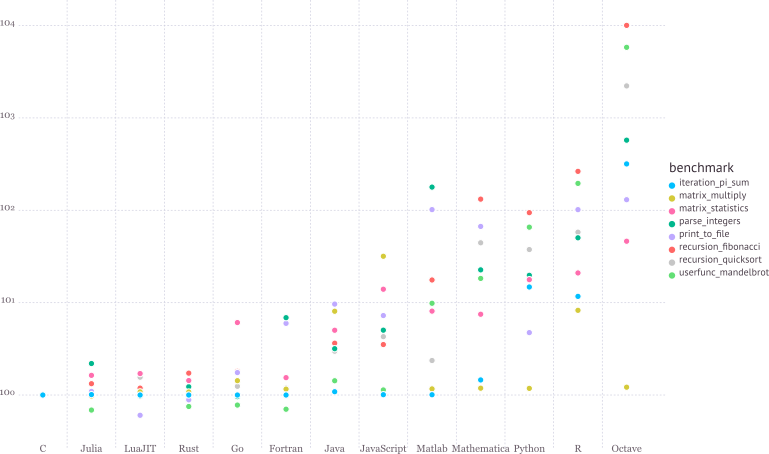
See https://julialang.org/benchmarks/ for the details of benchmark.
Write high-level, abstract code that closely resembles mathematical formulas
- yet produces fast, low-level machine code that has traditionally only been generated by static languages.
Julia is more than just "Fast R" or "Fast Matlab"
- Performance comes from features that work well together.
- You can't just take the magic dust that makes Julia fast and sprinkle it on [language of choice]
Learning resources
The (free) online course Introduction to Julia, by Jane Herriman.
Cheat sheet: The Fast Track to Julia.
Browse the Julia documentation.
For Matlab users, read Noteworthy Differences From Matlab.
For R users, read Noteworthy Differences From R.
For Python users, read Noteworthy Differences From Python.
The Learning page on Julia's website has pointers to many other learning resources.
Julia REPL (Read-Evaluation-Print-Loop)
The Julia REPL, or Julia shell, has at least five modes.
Default mode is the Julian prompt
julia>. Type backspace in other modes to enter default mode.Help mode
help?>. Type?to enter help mode.?search_termdoes a fuzzy search forsearch_term.Shell mode
shell>. Type;to enter shell mode.Package mode
(@v1.7) pkg>. Type]to enter package mode for managing Julia packages (install, uninstall, update, ...).Search mode
(reverse-i-search). Pressctrl+Rto enter search model.With
RCall.jlpackage installed, we can enter the R mode by typing$(shift+4) at Julia REPL.
Some survival commands in Julia REPL:
exit()orCtrl+D: exit Julia.Ctrl+C: interrupt execution.Ctrl+L: clear screen.Append
;(semi-colon) to suppress displaying output from a command. Same as Matlab.include("filename.jl")to source a Julia code file.
Seek help
Online help from REPL:
?function_name.Google.
Julia documentation: https://docs.julialang.org/en/.
Look up source code:
@edit sin(π).Discourse: https://discourse.julialang.org.
Friends.
Which IDE?
Julia homepage lists many choices: Juno, VS Code, Vim, ...
Unfortunately at the moment there are no mature RStudio- or Matlab-like IDE for Julia yet.
For dynamic document, e.g., homework, I recommend Jupyter Notebook or JupyterLab.
For extensive Julia coding, myself has been happily using the editor VS Code with extensions
JuliaandVS Code Jupyter Notebook Previewerinstalled.
Julia package system
Each Julia package is a Git repository. Each Julia package name ends with
.jl. E.g.,Distributions.jlpackage lives at https://github.com/JuliaStats/Distributions.jl.
Google search withPackageName.jlusually leads to the package on github.com.The package ecosystem is rapidly maturing; a complete list of registered packages (which are required to have a certain level of testing and documentation) is at http://pkg.julialang.org/.
For example, the package called
Distributions.jlis added with# in Pkg mode (@v1.7) pkg> add Distributions
and "removed" (although not completely deleted) with
# in Pkg mode
(@v1.7) pkg> rm Distributions
The package manager provides a dependency solver that determines which packages are actually required to be installed.
Non-registered packages are added by cloning the relevant Git repository. E.g.,
# in Pkg mode
(@v1.7) pkg> add https://github.com/OpenMendel/SnpArrays.jl
A package needs only be added once, at which point it is downloaded into your local
.julia/packagesdirectory in your home directory.
readdir(Sys.islinux() ? ENV["JULIA_PATH"] * "/pkg/packages" : ENV["HOME"] * "/.julia/packages")
- Directory of a specific package can be queried by
pathof():
using Distributions

pathof(Distributions)
If you start having problems with packages that seem to be unsolvable, you may try just deleting your .julia directory and reinstalling all your packages.
Periodically, one should run
updatein Pkg mode, which checks for, downloads and installs updated versions of all the packages you currently have installed.statuslists the status of all installed packages.Using functions in package.
using Distributions
This pulls all of the exported functions in the module into your local namespace, as you can check using the
whos()command. An alternative isimport Distributions
Now, the functions from the Distributions package are available only using
Distributions.<FUNNAME>
All functions, not only exported functions, are always available like this.
using RCall
x = randn(1000)
# $ is the interpolation operator
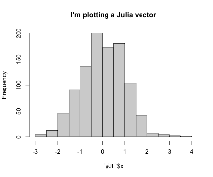
R"""
hist($x, main="I'm plotting a Julia vector")
"""
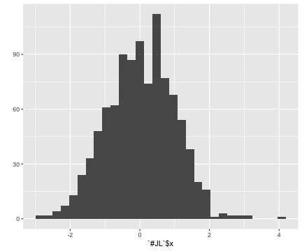
R"""
library(ggplot2)
qplot($x)
"""
x = R"""
rnorm(10)
"""
# collect R variable into Julia workspace
y = collect(x)
Access Julia variables in R REPL mode:
julia> x = rand(5) # Julia variable
R> y <- $x
Pass Julia expression in R REPL mode:
R> y <- $(rand(5))
Put Julia variable into R environment:
julia> @rput x
R> x
Get R variable into Julia environment:
R> r <- 2
Julia> @rget r
If you want to call Julia within R, check out the
JuliaCallpackage.
Some basic Julia code
# an integer, same as int in R
y = 1
# query type of a Julia object
typeof(y)
# a Float64 number, same as double in R
y = 1.0
typeof(y)
# Greek letters:  `\pi<tab>`
π
typeof(π)
# Greek letters:  `\theta<tab>`
θ = y + π
# emoji! `\:kissing_cat:<tab>`
😽 = 5.0
😽 + 1
# `\alpha<tab>\hat<tab>`
α̂ = π
For a list of unicode symbols that can be tab-completed, see https://docs.julialang.org/en/v1/manual/unicode-input/. Or in the help mode, type ? followed by the unicode symbol you want to input.
# vector of Float64 0s
x = zeros(5)
# vector Int64 0s
x = zeros(Int, 5)
# matrix of Float64 0s
x = zeros(5, 3)
# matrix of Float64 1s
x = ones(5, 3)
# define array without initialization
x = Matrix{Float64}(undef, 5, 3)
# fill a matrix by 0s
fill!(x, 0)
# initialize an array to be constant 2.5
fill(2.5, (5, 3))
# rational number
a = 3//5
typeof(a)
b = 3//7
a + b
# uniform [0, 1) random numbers
x = rand(5, 3)
# uniform random numbers (in single precision)
x = rand(Float16, 5, 3)
# random numbers from {1,...,5}
x = rand(1:5, 5, 3)
# standard normal random numbers
x = randn(5, 3)
# range
1:10
typeof(1:10)
1:2:10
typeof(1:2:10)
# integers 1-10
x = collect(1:10)
# or equivalently
[1:10...]
# Float64 numbers 1-10
x = collect(1.0:10)
# convert to a specific type
convert(Vector{Float64}, 1:10)
Matrices and vectors
Dimensions
x = randn(5, 3)
size(x)
size(x, 1) # nrow() in R
size(x, 2) # ncol() in R
# total number of elements
length(x)
Indexing
# 5 × 5 matrix of random Normal(0, 1)
x = randn(5, 5)
# first column
x[:, 1]
# first row
x[1, :]
# sub-array
x[1:2, 2:3]
# getting a subset of a matrix creates a copy, but you can also create "views"
z = view(x, 1:2, 2:3)
# same as
@views z = x[1:2, 2:3]
# change in z (view) changes x as well
z[2, 2] = 0.0
x
# y points to same data as x
y = x
# x and y point to same data
pointer(x), pointer(y)
# changing y also changes x
y[:, 1] .= 0
x
# create a new copy of data
z = copy(x)
pointer(x), pointer(z)
Concatenate matrices
# 3-by-1 vector
[1, 2, 3]
# 1-by-3 array
[1 2 3]
# multiple assignment by tuple
x, y, z = randn(5, 3), randn(5, 2), randn(3, 5)
[x y] # 5-by-5 matrix
[x y; z] # 8-by-5 matrix
Dot operation
Dot operation in Julia is elementwise operation, similar to Matlab.
x = randn(5, 3)
y = ones(5, 3)
x .* y # same x * y in R
x .^ (-2)
sin.(x)
Basic linear algebra
x = randn(5)
using LinearAlgebra
# vector L2 norm
norm(x)
# same as
sqrt(sum(abs2, x))
y = randn(5) # another vector
# dot product
dot(x, y) # x' * y
# same as
x'y
x, y = randn(5, 3), randn(3, 2)
# matrix multiplication, same as %*% in R
x * y
x = randn(3, 3)
# conjugate transpose
x'
b = rand(3)
x'b # same as x' * b
# trace
tr(x)
det(x)
rank(x)
Sparse matrices
using SparseArrays

# 10-by-10 sparse matrix with sparsity 0.1
X = sprandn(10, 10, .1)
# dump() in Julia is like str() in R
dump(X)
# convert to dense matrix; be cautious when dealing with big data
Xfull = convert(Matrix{Float64}, X)
# convert a dense matrix to sparse matrix
sparse(Xfull)
# syntax for sparse linear algebra is same as dense linear algebra
β = ones(10)
X * β
# many functions apply to sparse matrices as well
sum(X)
Control flow and loops
- if-elseif-else-end
if condition1
    # do something
elseif condition2
    # do something
else
    # do something
end
forloop
for i in 1:10
    println(i)
end
- Nested
forloop:
for i in 1:10
    for j in 1:5
        println(i * j)
    end
end
Same as
for i in 1:10, j in 1:5
    println(i * j)
end
- Exit loop:
for i in 1:10
    # do something
    if condition1
        break # skip remaining loop
    end
end
- Exit iteration:
for i in 1:10
    # do something
    if condition1
        continue # skip to next iteration
    end
    # do something
end
Functions
In Julia, all arguments to functions are passed by reference, in contrast to R and Matlab.
Function names ending with
!indicates that function mutates at least one argument, typically the first.sort!(x) # vs sort(x)
Function definition
function func(req1, req2; key1=dflt1, key2=dflt2)
    # do stuff
    return out1, out2, out3
end
Required arguments are separated with a comma and use the positional notation.
Optional arguments need a default value in the signature.
Semicolon is not required in function call.
return statement is optional.
Multiple outputs can be returned as a tuple, e.g., return out1, out2, out3.
Anonymous functions, e.g.,
x -> x^2, is commonly used in collection function or list comprehensions.map(x -> x^2, y) # square each element in x
Functions can be nested:
function outerfunction()
    # do some outer stuff
    function innerfunction()
        # do inner stuff
        # can access prior outer definitions
    end
    # do more outer stuff
end
- Functions can be vectorized using the Dot syntax:
# defined for scalar
function myfunc(x)
    return sin(x^2)
end

x = randn(5, 3)
myfunc.(x)
Collection function (think this as the series of
applyfunctions in R).Apply a function to each element of a collection:
map(f, coll) # or
map(coll) do elem
    # do stuff with elem
    # must contain return
end
map(x -> sin(x^2), x)
map(x) do elem
    elem = elem^2
    return sin(elem)
end
# Mapreduce
mapreduce(x -> sin(x^2), +, x)
# same as
sum(x -> sin(x^2), x)
- List comprehension
[sin(2i + j) for i in 1:5, j in 1:3] # similar to Python
Type system
Every variable in Julia has a type.
When thinking about types, think about sets.
Everything is a subtype of the abstract type
Any.An abstract type defines a set of types
- Consider types in Julia that are a
Number:
- Consider types in Julia that are a
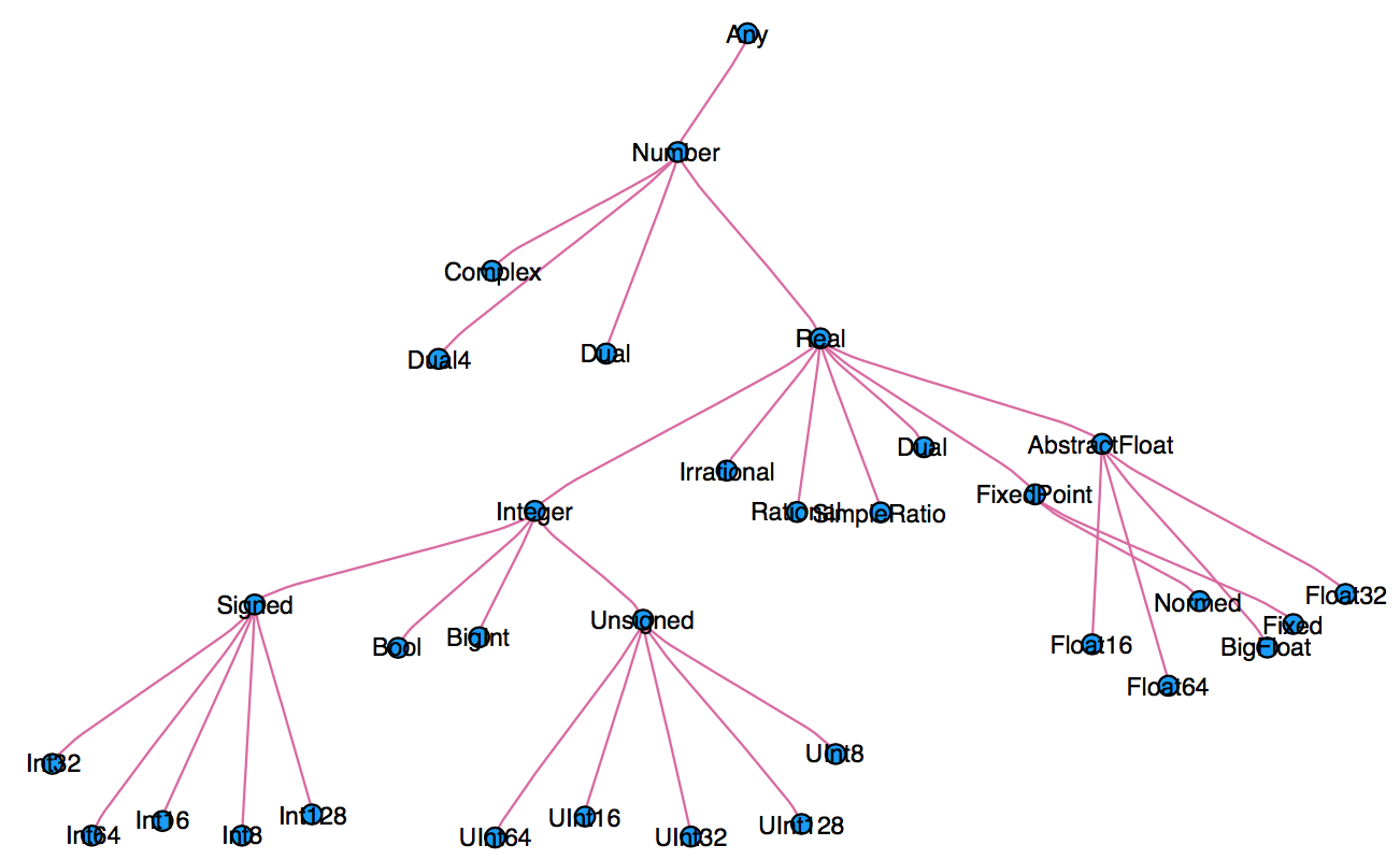
- We can explore type hierarchy with
typeof(),supertype(), andsubtypes().
typeof(1.0), typeof(1)
supertype(Float64)
subtypes(AbstractFloat)
# Is Float64 a subtype of AbstractFloat?
Float64 <: AbstractFloat
# On 64bit machine, Int == Int64
Int == Int64
# convert to Float64
convert(Float64, 1)
# same as
Float64(1)
# Float32 vector
x = randn(Float32, 5)
# convert to Float64
convert(Vector{Float64}, x)
# same as
Float64.(x)
# convert Float64 to Int64
convert(Int, 1.0)
convert(Int, 1.5) # should use round(1.5)
round(Int, 1.5)
Multiple dispatch
Multiple dispatch lies in the core of Julia design. It allows built-in and user-defined functions to be overloaded for different combinations of argument types.
Let's consider a simple "doubling" function:
g(x) = x + x
g(1.5)
This definition is too broad, since some things, e.g., strings, can't be added
g("hello world")
- This definition is correct but too restrictive, since any
Numbercan be added.
g(x::Float64) = x + x
- This definition will automatically work on the entire type tree above!
g(x::Number) = x + x
This is a lot nicer than
function g(x)
    if isa(x, Number)
        return x + x
    else
        throw(ArgumentError("x should be a number"))
    end
end
methods(func)function display all methods defined forfunc.
methods(g)
When calling a function with multiple definitions, Julia will search from the narrowest signature to the broadest signature.
@which func(x)marco tells which method is being used for argument signaturex.
# an Int64 input
@which g(1)
# a Vector{Float64} input
@which g(randn(5))
Just-in-time compilation (JIT)
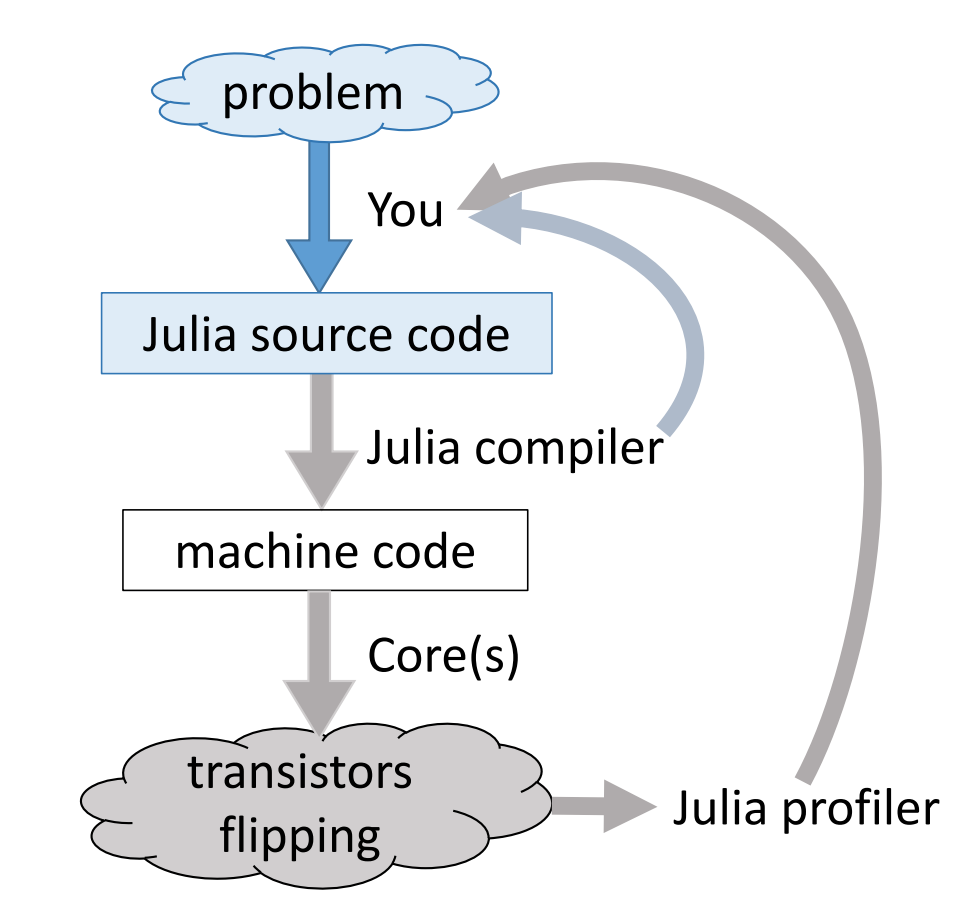
Following figures are taken from Arch D. Robinson's slides Introduction to Writing High Performance Julia.
 |
 |
|---|---|
Julia's efficiency results from its capability to infer the types of all variables within a function and then call LLVM to generate optimized machine code at run-time.
Consider the g (doubling) function defined earlier. This function will work on any type which has a method for +.
g(2), g(2.0)
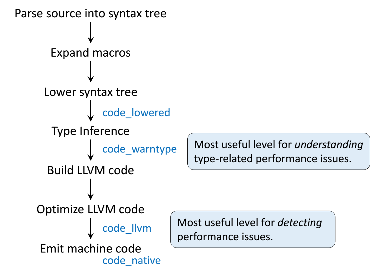
Step 1: Parse Julia code into abstract syntax tree (AST).
@code_lowered g(2)
Step 2: Type inference according to input type.
@code_warntype g(2)
@code_warntype g(2.0)
Step 3: Compile into LLVM bytecode (equivalent of R bytecode generated by the compiler package).
@code_llvm g(2)
@code_llvm g(2.0)
We didn't provide a type annotation. But different LLVM code was generated depending on the argument type!
In R or Python, g(2) and g(2.0) would use the same code for both.
In Julia, g(2) and g(2.0) dispatches to optimized code for Int64 and Float64, respectively.
For integer input x, LLVM compiler is smart enough to know x + x is simple shifting x by 1 bit, which is faster than addition.
- Step 4: Lowest level is the assembly code, which is machine dependent.
@code_native g(2)
@code_native g(2.0)
Profiling Julia code
Julia has several built-in tools for profiling. The @time marco outputs run time and heap allocation.
# a function defined earlier
function tally(x::Array)
    s = zero(eltype(x))
    for v in x
        s += v
    end
    s
end

using Random
Random.seed!(123)
a = rand(20_000_000)
@time tally(a) # first run: include compile time
@time tally(a)
For more robust benchmarking, the BenchmarkTools.jl package is highly recommended.
using BenchmarkTools

@benchmark tally($a)
The Profile module gives line by line profile results.
using Profile

Profile.clear()
@profile tally(a)
Profile.print(format=:flat)
One can use ProfileView package for better visualization of profile data:
using ProfileView

ProfileView.view()
# check type stability
@code_warntype tally(a)
# check LLVM bitcode
@code_llvm tally(a)
@code_native tally(a)
Exercise: Annotate the loop in tally function by @simd and look for the difference in LLVM bitcode and machine code.
Memory profiling
Detailed memory profiling requires a detour. First let's write a script bar.jl, which contains the workload function tally and a wrapper for profiling.
;cat bar.jl
Next, in terminal, we run the script with --track-allocation=user option.
#;julia --track-allocation=user bar.jl
The profiler outputs a file bar.jl.51116.mem.
;cat bar.jl.51116.mem