Computer Languages (R, Python, Julia, C/C++)
System information (for reproducibility)
versioninfo()
# load packages
using BenchmarkTools, Distributions, Libdl, PyCall, Random, RCall, Statistics
Types of computer languages
Compiled languages (low-level languages): C/C++, Fortran, ...
- Directly compiled to machine code that is executed by CPU
- Pros: fast, memory efficient
- Cons: longer development time, hard to debug
Interpreted language (high-level languages): R, Matlab, Python, SAS IML, JavaScript, ...
- Interpreted by interpreter
- Pros: fast prototyping
- Cons: excruciatingly slow for loops
Mixed (dynamic) languages: Matlab (JIT), R (
compilerpackage), Julia, Cython, JAVA, ...- Pros and cons: between the compiled and interpreted languages
Script languages: Linux shell scripts, Perl, ...
- Extremely useful for some data preprocessing and manipulation
Database languages: SQL, Hive (Hadoop).
- Data analysis never happens if we do not know how to retrieve data from databases
203B (Introduction to Data Science) covers some basics on scripting and database.
How high-level languages work?
Comics: The Life of a Bytecode Language
- Typical execution of a high-level language such as R, Python, and Matlab.
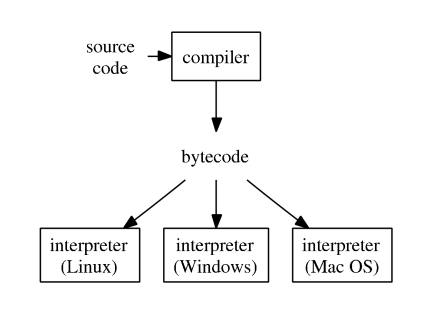
To improve efficiency of interpreted languages such as R or Matlab, conventional wisdom is to avoid loops as much as possible. Aka, vectorize code
The only loop you are allowed to have is that for an iterative algorithm.
When looping is unavoidable, need to code in C, C++, or Fortran. This creates the notorious two language problem
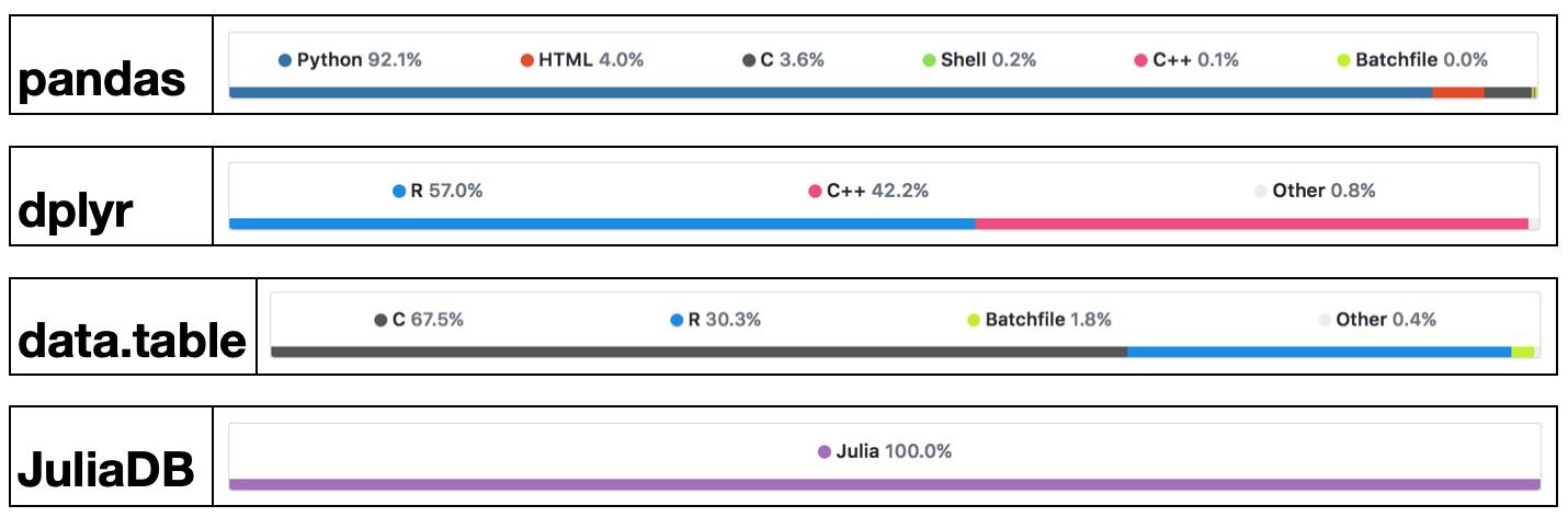
Success stories: the popularglmnetpackage in R is coded in Fortran;tidyverseanddata.tablepackages use a lot RCpp/C++.
High-level languages have made many efforts to bring themselves closer to the performance of low-level languages such as C, C++, or Fortran, with a variety levels of success.
- Matlab has employed JIT (just-in-time compilation) technology since 2002.
- Since R 3.4.0 (Apr 2017), the JIT bytecode compiler is enabled by default at its level 3.
- Cython is a compiler system based on Python.
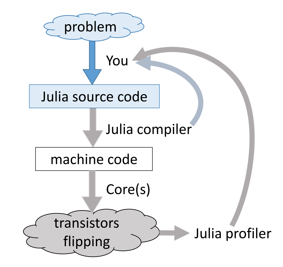
Modern languages such as Julia tries to solve the two language problem. That is to achieve efficiency without vectorizing code.
Julia execution.
Gibbs sampler example by Doug Bates
Doug Bates (member of R-Core, author of popular R packages
Matrix,lme4,RcppEigen, etc)As some of you may know, I have had a (rather late) mid-life crisis and run off with another language called Julia.
-- Doug Bates (on the `knitr` Google Group)
An example from Dr. Doug Bates's slides Julia for R Programmers.
The task is to create a Gibbs sampler for the density
$$ f(x, y) = k x^2 exp(- x y^2 - y^2 + 2y - 4x), x > 0 $$ using the conditional distributions $$ \begin{eqnarray*} X | Y &\sim& \Gamma \left( 3, \frac{1}{y^2 + 4} \right) \\ Y | X &\sim& N \left(\frac{1}{1+x}, \frac{1}{2(1+x)} \right). \end{eqnarray*} $$
- R solution. The
RCall.jlpackage allows us to execute R code without leaving theJuliaenvironment. We first define an R functionRgibbs().
# show R information
R"""
sessionInfo()
"""
# define a function for Gibbs sampling

R"""
library(Matrix)

Rgibbs <- function(N, thin) {
  mat <- matrix(0, nrow=N, ncol=2)
  x <- y <- 0
  for (i in 1:N) {
    for (j in 1:thin) {
      x <- rgamma(1, 3, y * y + 4) # 3rd arg is rate
      y <- rnorm(1, 1 / (x + 1), 1 / sqrt(2 * (x + 1)))
    }
    mat[i,] <- c(x, y)
  }
  mat
}
"""
To generate a sample of size 10,000 with a thinning of 500. How long does it take?
R"""
system.time(Rgibbs(10000, 500))
"""
- This is a Julia function for the same Gibbs sampler:
function jgibbs(N, thin)
    mat = zeros(N, 2)
    x = y = 0.0
    for i in 1:N
        for j in 1:thin
            x = rand(Gamma(3, 1 / (y * y + 4)))
            y = rand(Normal(1 / (x + 1), 1 / sqrt(2(x + 1))))
        end
        mat[i, 1] = x
        mat[i, 2] = y
    end
    mat
end
Generate the same number of samples. How long does it take?
jgibbs(100, 5); # warm-up
@elapsed jgibbs(10000, 500)
We see 40-80 fold speed up of Julia over R on this example, with similar coding effort!
Comparing C, R, Python, and Julia
To better understand how these languages work, we consider a simple task: summing a vector.
Let's first generate data: 1 million double precision numbers from uniform [0, 1].
Random.seed!(123) # seed
x = rand(1_000_000) # 1 million random numbers in [0, 1)
sum(x)
In this class, we use package BenchmarkTools.jl for robust benchmarking. It's analog of microbenchmark or bench package in R.
C
We would use the low-level C code as the baseline for copmarison. In Julia, we can easily run compiled C code using the ccall function.
using Libdl

C_code = """
#include <stddef.h>
double c_sum(size_t n, double *X) {
    double s = 0.0;
    for (size_t i = 0; i < n; ++i) {
        s += X[i];
    }
    return s;
}
"""

const Clib = tempname()   # make a temporary file

# compile to a shared library by piping C_code to gcc
# (works only if you have gcc installed):

open(`gcc -std=c99 -fPIC -O3 -msse3 -xc -shared -o $(Clib * "." * Libdl.dlext) -`, "w") do f
    print(f, C_code)
end

# define a Julia function that calls the C function:
c_sum(X::Array{Float64}) = ccall(("c_sum", Clib), Float64, (Csize_t, Ptr{Float64}), length(X), X)
# make sure it gives same answer
c_sum(x)
# dollar sign to interpolate array x into local scope for benchmarking
bm = @benchmark c_sum($x)
benchmark_result = Dict() # a dictionary to store median runtime (in milliseconds)

# store median runtime (in milliseconds)
benchmark_result["C"] = median(bm.times) / 1e6
R, buildin sum
Next we compare to the build in sum function in R, which is implemented using C.
R"""
library(bench)
y <- $x
rbm_builtin <- bench::mark(sum(y))
"""
# store median runtime (in milliseconds)
@rget rbm_builtin # dataframe
benchmark_result["R builtin"] = median(rbm_builtin[!, :median]) * 1000
R, handwritten loop
Handwritten loop in R is much slower.
R"""
sum_r <- function(x) {
  s <- 0
  for (xi in x) {
    s <- s + xi
  }
  s
}
library(bench)
y <- $x
rbm_loop <- bench::mark(sum_r(y))
"""
# store median runtime (in milliseconds)
@rget rbm_loop # dataframe
benchmark_result["R loop"] = median(rbm_loop[!, :median]) * 1000
R, Rcpp
Rcpp package is the easiest way to incorporate C++ code in R.
R"""
library(Rcpp)

cppFunction('double rcpp_sum(NumericVector x) {
  int n = x.size();
  double total = 0;
  for(int i = 0; i < n; ++i) {
    total += x[i];
  }
  return total;
}')
rcpp_sum
"""
R"""
rbm_rcpp <- bench::mark(rcpp_sum(y))
"""
# store median runtime (in milliseconds)
@rget rbm_rcpp # dataframe
benchmark_result["R Rcpp"] = median(rbm_rcpp[!, :median]) * 1000
Python, builtin sum
Built in function sum in Python.
PyCall.pyversion
# get the Python built-in "sum" function:
pysum = pybuiltin("sum")
bm = @benchmark $pysum($x)
# store median runtime (in miliseconds)
benchmark_result["Python builtin"] = median(bm.times) / 1e6
Python, handwritten loop
py"""
def py_sum(A):
    s = 0.0
    for a in A:
        s += a
    return s
"""

sum_py = py"py_sum"

bm = @benchmark $sum_py($x)
# store median runtime (in miliseconds)
benchmark_result["Python loop"] = median(bm.times) / 1e6
Python, numpy
Numpy is the high-performance scientific computing library for Python.
# bring in sum function from Numpy
numpy_sum = pyimport("numpy")."sum"
bm = @benchmark $numpy_sum($x)
# store median runtime (in miliseconds)
benchmark_result["Python numpy"] = median(bm.times) / 1e6
Numpy performance is on a par with Julia build-in sum function. Both are about 3 times faster than C, possibly because of usage of SIMD.
Julia, builtin sum
@time, @elapsed, @allocated macros in Julia report run times and memory allocation.
@time sum(x) # no compilation time after first run
For more robust benchmarking, we use BenchmarkTools.jl package.
bm = @benchmark sum($x)
benchmark_result["Julia builtin"] = median(bm.times) / 1e6
Julia, handwritten loop
Let's also write a loop and benchmark.
function jl_sum(A)
    s = zero(eltype(A))
    for a in A
        s += a
    end
    s
end

bm = @benchmark jl_sum($x)
benchmark_result["Julia loop"] = median(bm.times) / 1e6
Exercise: annotate the loop by @simd and benchmark again.
Summary
sort(collect(benchmark_result), by = x -> x[2])
C,R builtinare the baseline C performance (gold standard).Python builtinandPython loopare 80-100 fold slower than C because the loop is interpreted.R loopis about 30 folder slower than C and indicates the performance of JIT bytecode generated by its compiler package (turned on by default since R v3.4.0 (Apr 2017)).Julia loopis close to C performance, because Julia code is JIT compiled.Julia builtinandPython numpyare 3-4 folder faster than C because of SIMD.
Take home message for computational scientists
High-level language (R, Python, Matlab) programmers should be familiar with existing high-performance packages. Don't reinvent wheels.
- R: RcppEigen, tidyverse, ...
- Python: numpy, scipy, ...
In most research projects, looping is unavoidable. Then we need to use a low-level language.
- R: Rcpp, ...
- Python: Cython, ...
In this course, we use Julia, which seems to circumvent the two language problem. So we can spend more time on algorithms, not on juggling $\ge 2$ languages.