Biostat 257 Homework 2
Due Apr 29 @ 11:59PM
versioninfo()
# load libraries
using BenchmarkTools, DelimitedFiles, Images, LinearAlgebra, Random
Q1. Nonnegative Matrix Factorization
Nonnegative matrix factorization (NNMF) was introduced by Lee and Seung (1999) as an analog of principal components and vector quantization with applications in data compression and clustering. In this homework we consider algorithms for fitting NNMF and (optionally) high performance computing using graphical processing units (GPUs).
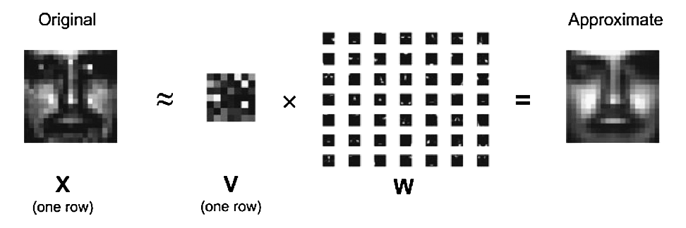
In mathematical terms, one approximates a data matrix $\mathbf{X} \in \mathbb{R}^{m \times n}$ with nonnegative entries $x_{ij}$ by a product of two low-rank matrices $\mathbf{V} \in \mathbb{R}^{m \times r}$ and $\mathbf{W} \in \mathbb{R}^{r \times n}$ with nonnegative entries $v_{ik}$ and $w_{kj}$. Consider minimization of the squared Frobenius norm $$ L(\mathbf{V}, \mathbf{W}) = \|\mathbf{X} - \mathbf{V} \mathbf{W}\|_{\text{F}}^2 = \sum_i \sum_j \left(x_{ij} - \sum_k v_{ik} w_{kj} \right)^2, \quad v_{ik} \ge 0, w_{kj} \ge 0, $$ which should lead to a good factorization. Lee and Seung suggest an iterative algorithm with multiplicative updates $$ v_{ik}^{(t+1)} = v_{ik}^{(t)} \frac{\sum_j x_{ij} w_{kj}^{(t)}}{\sum_j b_{ij}^{(t)} w_{kj}^{(t)}}, \quad \text{where } b_{ij}^{(t)} = \sum_k v_{ik}^{(t)} w_{kj}^{(t)}, $$ $$ w_{kj}^{(t+1)} = w_{kj}^{(t)} \frac{\sum_i x_{ij} v_{ik}^{(t+1)}}{\sum_i b_{ij}^{(t+1/2)} v_{ik}^{(t+1)}}, \quad \text{where } b_{ij}^{(t+1/2)} = \sum_k v_{ik}^{(t+1)} w_{kj}^{(t)} $$ that will drive the objective $L^{(t)} = L(\mathbf{V}^{(t)}, \mathbf{W}^{(t)})$ downhill. Superscript $t$ indicates iteration number. In following questions, efficiency (both speed and memory) will be the most important criterion when grading this problem.
Q1.1 Develop code
Implement the algorithm with arguments: $\mathbf{X}$ (data, each row is a vectorized image), rank $r$, convergence tolerance, and optional starting point.
function nnmf(
    X       :: Matrix{T},
    r       :: Integer;
    maxiter :: Integer = 1000,
    tolfun  :: Number = 1e-4,
    V       :: Matrix{T} = rand(T, size(X, 1), r),
    W       :: Matrix{T} = rand(T, r, size(X, 2))
    ) where T <: AbstractFloat
    # implementation
    # Output
    V, W, obj, niter
end
Q1.2 Data
Database 1 from the MIT Center for Biological and Computational Learning (CBCL) reduces to a matrix $\mathbf{X}$ containing $m = 2,429$ gray-scale face images with $n = 19 \times 19 = 361$ pixels per face. Each image (row) is scaled to have mean and standard deviation 0.25.
Read in the nnmf-2429-by-361-face.txt file, e.g., using readdlm function, and display a couple sample images, e.g., using the Images.jl package.
X = readdlm("nnmf-2429-by-361-face.txt")
colorview(Gray, reshape(X[1, :], 19, 19))
colorview(Gray, reshape(X[5, :], 19, 19))
Q1.3 Correctness and efficiency
Report the run times, using @time, of your function for fitting NNMF on the MIT CBCL face data set at ranks $r=10, 20, 30, 40, 50$. For ease of comparison (and grading), please start your algorithm with the provided $\mathbf{V}^{(0)}$ (first $r$ columns of V0.txt) and $\mathbf{W}^{(0)}$ (first $r$ rows of W0.txt) and stopping criterion
$$
\frac{|L^{(t+1)} - L^{(t)}|}{|L^{(t)}| + 1} \le 10^{-4}.
$$
Hint: When I run the following code using my own implementation of nnmf
for r in [10, 20, 30, 40, 50]
    println("r=$r")
    V0 = V0full[:, 1:r]
    W0 = W0full[1:r, :]
    @time V, W, obj, niter = nnmf(X, r; V = V0, W = W0)
    println("obj=$obj, niter=$niter")
end
the output is
r=10
  1.047598 seconds (20 allocations: 6.904 MiB)
obj=11730.38800985483, niter=239
r=20
  1.913147 seconds (20 allocations: 7.120 MiB)
obj=8497.222317850326, niter=394
r=30
  2.434662 seconds (20 allocations: 7.336 MiB)
obj=6621.627345486279, niter=482
r=40
  3.424469 seconds (22 allocations: 7.554 MiB)
obj=5256.663870563529, niter=581
r=50
  4.480342 seconds (23 allocations: 7.774 MiB)
obj=4430.201581697291, niter=698
Since my laptop is about 6-7 years old, I expect to see your run time shorter than mine. Your memory allocation should be less or equal to mine.
Q1.4 Non-uniqueness
Choose an $r \in \{10, 20, 30, 40, 50\}$ and start your algorithm from a different $\mathbf{V}^{(0)}$ and $\mathbf{W}^{(0)}$. Do you obtain the same objective value and $(\mathbf{V}, \mathbf{W})$? Explain what you find.
Q1.5 Fixed point
For the same $r$, start your algorithm from $v_{ik}^{(0)} = w_{kj}^{(0)} = 1$ for all $i,j,k$. Do you obtain the same objective value and $(\mathbf{V}, \mathbf{W})$? Explain what you find.
Q1.6 Interpret NNMF result
Plot the basis images (rows of $\mathbf{W}$) at rank $r=50$. What do you find?
Q1.7 GPU (optional)
Investigate the GPU capabilities of Julia. Report the speed gain of your GPU code over CPU code at ranks $r=10, 20, 30, 40, 50$. Make sure to use the same starting point as in Q1.3.
Q2. Estimating Kinship Matrix
Consider the numerical task of estimating an $n \times n$ kinship matrix $\Phi$ from an $n \times m$ genotype matrix $\mathbf{G}$. Here $n$ is the number of individuals and $m$ is the number of genetic markers. Lange et al derived a method of moment estimator of form $$ \widehat \Phi_{ij} = \frac{e_{ij} - \sum_{k=1}^m [p_k^2 + (1 - p_k)^2]}{m - \sum_{k=1}^m [p_k^2 + (1 - p_k)^2]}, \quad 1 \le i, j \le n, $$ where $$ \begin{eqnarray*} e_{ij} &=& \frac{1}{4} \sum_{k=1}^m [g_{ik} g_{jk} + (2 - g_{ik})(2 - g_{jk})] \\ p_k &=& \frac {1}{2n} \sum_{i=1}^n g_{ik}. \end{eqnarray*} $$
Q2.1 Develop code
Write a function that takes a matrix G as input and outputs the method of moment estimator.
Make your function as efficient (both speed and memory) as possible.
function kinship(G::Matrix{T}) where T <: AbstractFloat
    n, m = size(G)
    # TODO: your code here
    Φ = zeros(n, m)
    # output
    Φ
end
Q2.2 Correctness
First let's make sure our function yields correct answer. Run your function on a fake genotype matrix
# generate a fake genotype matrix with entries {0, 1, 2}
Random.seed!(257)
G = rand(0.0:2.0, 1000, 10000)
Φ = kinship(G)
Compare the upper left $5 \times 5$ block to what I got using my implementation
Φ[1:5, 1:5]
5×5 Matrix{Float64}:
  0.673584     -0.000762864  -0.00266412   0.00343992   0.00293959
 -0.000762864   0.665178     -0.0101691   -0.0110697    0.00223912
 -0.00266412   -0.0101691     0.665078     0.0102444    0.00253932
  0.00343992   -0.0110697     0.0102444    0.66768     -0.0083679
  0.00293959    0.00223912    0.00253932  -0.0083679    0.663777
Q2.3 Efficiency
In a typical genetic data set, $n$ is at order of $10^3 \sim 10^6$ and $m$ is at order of $10^6 \sim 10^7$. Benchmark your function using the smaller data set $G$ generated in Q2.2. Efficiency (both speed and memory) will be the most important criterion when grading this question.
# benchmark
@btime kinship($G)
Hint: I got @btime output
82.144 ms (3 allocations: 7.64 MiB)